Forecasting Reservoir Water Levels Using Deep Neural Networks: A Case Study of Angat Dam in the Philippines

Abstract

Forecasting reservoir water levels is essential in water supply management, impacting both operations and intervention strategies. This paper examines the short-term and long-term forecasting performance of several statistical and machine learning-based methods for predicting the water levels of the Angat Dam in the Philippines. A total of six forecasting methods are compared: naïve/persistence; seasonal mean; autoregressive integrated moving average (ARIMA); gradient boosting machines (GBM); and two deep neural networks (DNN) using a long short-term memory-based (LSTM) encoder-decoder architecture: a univariate model (DNN-U) and a multivariate model (DNN-M). Daily historical water levels from 2001 to 2021 are used in predicting future water levels. In addition, we include meteorological data (rainfall and the Oceanic Niño Index) and irrigation data as exogenous variables. To evaluate the forecast accuracy of our methods, we use a time series cross-validation approach to establish a more robust estimate of the error statistics. Our results show that our DNN-U model has the best accuracy in the 1-day-ahead scenario with a mean absolute error (MAE) and root mean square error (RMSE) of 0.2 m. In the 30-day-, 90-day-, and 180-day-ahead scenarios, the DNN-M shows the best performance with MAE (RMSE) scores of 2.9 (3.3), 5.1 (6.0), and 6.7 (8.1) meters, respectively. Additionally, we demonstrate that further improvements in performance are possible by scanning over all possible combinations of the exogenous variables and only using a subset of them as features. In summary, we provide a comprehensive framework for evaluating water level forecasting by defining a baseline accuracy, analyzing performance across multiple prediction horizons, using time series cross-validation to assess accuracy and uncertainty, and examining the effects of exogenous variables on forecasting performance. In the process, our work addresses several notable gaps in the methodologies of previous works.

1. Introduction

In 2019, Metro Manila, the economic and cultural center of the Philippines and home to a population of over 12 million, suffered one the worst water shortage crises in the past decade [1]. Low water levels in nearby reservoirs triggered daily rotational service interruptions, forcing residents to line up daily to meet their water consumption needs. In order to better address this problem in the future, we believe that more robust forecasting methodologies should be developed for the use of the various water resource managers and agencies in the Philippines. This study was initiated to aid in the forecasting of water levels in the dams that supply water to Metro Manila, with the final goal of full implementation and adoption of the methods described in this work.

Dams and reservoirs play a crucial role in water resource management. Not only are they used to supply water to urban areas, they are also used for flood control, irrigation for farmland areas, and in the generation of hydroelectric power. To maintain the optimal performance of a multipurpose water storage facility, the reservoir or dam level needs to be continuously monitored so that necessary adjustments can be made in a timely manner.

However, forecasting water levels happens to be one of the more challenging tasks for operators and planners in the water supply management domain. Although water levels mainly depend on the inflows to the reservoir and outflow releases for purposes such as water consumption, irrigation, hydroelectric power, etc., there may be uncertainties in other related variables, such as long-term changes in the dynamics of rainfall and unforeseen fluctuations in consumer demand.

In its early days, the prediction of water levels relied on linear mathematical relationships based on the experience of the operators and rule curve guidelines derived from the analysis of historical inflows and climatology [2]. Recent decades have seen the introduction of machine learning (ML) models, allowing higher levels of accuracy since they are capable of capturing non-linearities in a dynamical system, which traditional models do not necessarily address. They are also advantageous in dealing with large amounts of data in terms of efficiency, accuracy, multi-dimensionality, scalability, and flexibility [3]. In addition, specific ML models can be trained to learn more efficient representations of complex non-linear relationships. This includes capturing the impact of the uncertainties in measuring watershed parameters, hydrological variables, and even operational decisions.

Recently, several works have examined the use of ML models for forecasting various features in the water resource management and hydrology research domains. These include studies in predicting dam inflow and runoff, as well as forecasting the water levels of lakes, reservoirs, and other bodies of water. In the case of dam operation and management, ML has been investigated as a means of generating reliable predictions in order to improve the safety of operations [4,5].

In a previous study, tree-based models, such as decision trees (DT), random forests (RF) and gradient boosted trees (GB), together with artificial neural networks (ANN) were used to forecast the dam inflow into the Soyang River Dam in South Korea [6]. The work demonstrated that an ensemble approach that combined the forecasts of RF/GB with a multilayer perceptron (MLP) could achieve a greater level of performance compared to using a single individual model. The predictive power of tree-based techniques is also highlighted in the case of the Upo wetland in South Korea, where RF was shown to have the best forecast accuracy when pitted against ANNs, DTs, and support vector machines (SVM) [7]. Other methods, such as the gaussian process (GP), multiple linear regression (MLR), and k-nearest neighbor (KNN), have also been compared to tree-based and ANN models in predicting the water level of Lake Erie [8]. Their results highlight how ML methods, specifically the MLR and M5P model tree, had higher accuracy and were much faster to train compared to the process-based advanced hydrologic prediction system (AHPS) [9].

Specific work has also been conducted that explores different neural network and deep learning (DL) architectures for forecasting water levels. In one study, two neural network models were made to generate forecasts for the water levels of 69 temperate lakes in Poland [10]. The results showed that a fully connected feed forward architecture slightly outperformed a deep neural network composed of autoencoder layers, convolution layers, and long short-term memory (LSTM) cells. Recurrent neural networks (RNN), specifically LSTM networks, have also been used in predicting the daily runoff of the Yichang and Hankou hydrological stations located along the Yangtze River [11]. The work combines seasonal and trend decomposition using Loess (STL) with neural networks and demonstrates that better performance can be achieved by using a time series decomposition method before applying the DL model. Finally, LSTM-based sequence-to-sequence (seq2seq) architectures have also been utilized to predict the two-day inflow rate of the Soyang River Dam [12]. The study provides a comprehensive ablation study of their proposed architecture and demonstrates how their model exhibits state-of-the-art accuracy by outperforming proposed models from other studies.

This paper presents a comprehensive framework for evaluating water level predictions that addresses several significant gaps in the methodology of the works outlined above.

First, while most of the works mentioned above focus on producing one-step forecasts, examining how well forecasting methods perform in multi-step forecasting scenarios is often more useful. Generating both short- and long-term forecasts provides more utility to the managers and operators of water resources in terms of strategic planning and intervention. A previous study that attempted to predict the water levels of a hydropower reservoir, in the Miño River in Spain, looked at statistical and ML-based techniques for both long-and short-term scenarios [13]. While a persistence-based approach using a typical year showcased high accuracy in the long-term when compared to detrended fluctuation analysis (DFA) and autoregressive moving average models (ARMA), a comparison with more established ML methods such as RF, GBM, SVM, and ANN was not examined in the long-term case. In contrast, our work uses the same collection of statistical and ML-based methods for all sets of prediction horizons.

Second, most of the previously mentioned studies used a single train-test partition for model evaluation. This approach provides a simple unbiased way to calculate the error metrics for time series forecasting, however it does not accurately capture how well the models generalize any unseen data. In most ML applications, cross-validation (CV) is the standard method for analyzing model performance. Most standard CV techniques, such as k-fold cross-validation, are typically inappropriate for time series data if applied without some modifications to the method. We propose using a time-series cross validation approach [14] to better understand how well each forecasting method generalizes any future data.

Third, we found that most of the cited works failed to include simple baseline methods, a common staple in forecasting competitions [15,16]. To properly gauge the relative performance of the ML models, we also include two simple forecasting methods as baselines, namely the naïve (also called the persistence method) and seasonal mean methods. This will allow the performance results to be better contextualized, especially regarding the relative complexity between models.

Finally, previous works tend to include explanatory/exogenous variables in the modeling process by default and often fail to examine if their addition provides positive (or negative) gains in performance. In fact, past competitions in time series forecasting have shown that additional variables are not necessarily helpful [17]. This work examines how prediction accuracy changes based on the inclusion of exogenous variables.

In summary, the novelty and innovation of this work lies with the consolidation of our proposed solutions for each of the shortcomings mentioned above into a single generalized framework:

• We provide an analysis of deep neural networks for both short-and long-term forecasting horizons using multiple exogenous variables;
• We propose the use of a time series cross-validation method in order to obtain more robust estimates of prediction accuracy;
• We include simple baseline methods, namely the naive/persistence and seasonal mean methods, in order to properly contextualize the relative performance of the more sophisticated models;
• We examine prediction accuracy based on the inclusion or exclusion of several related exogenous variables.

2. Models and Methodology

2.1. Study Area

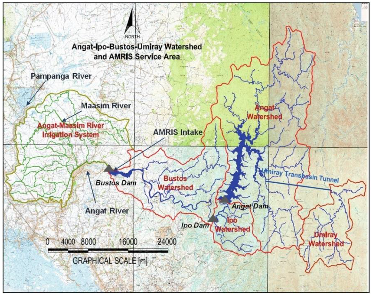
The Angat Dam and reservoir is located within the Angat Watershed Forest Reserve in Bulacan, Philippines shown in Figure 1. Construction of the facilities lasted from 1964 to 1967, and it became operational in 1968. The main inflow to the dam reservoir is the Angat River with three major tributaries: Talaguio River; Catmon River; and Matulid River. The Angat Dam is a multipurpose dam used for the water supply of residential and industrial consumers, farmland irrigation, flood control, and power generation. The dam supplies approximately 90% of Metro Manila’s (the capital region of the Philippines) potable water supply and irrigates 31,000 ha of farmland in the provinces of Pampanga and Bulacan [18]. The dam has an effective storage capacity of about 850,000,000 m³.

2.2. Data Description

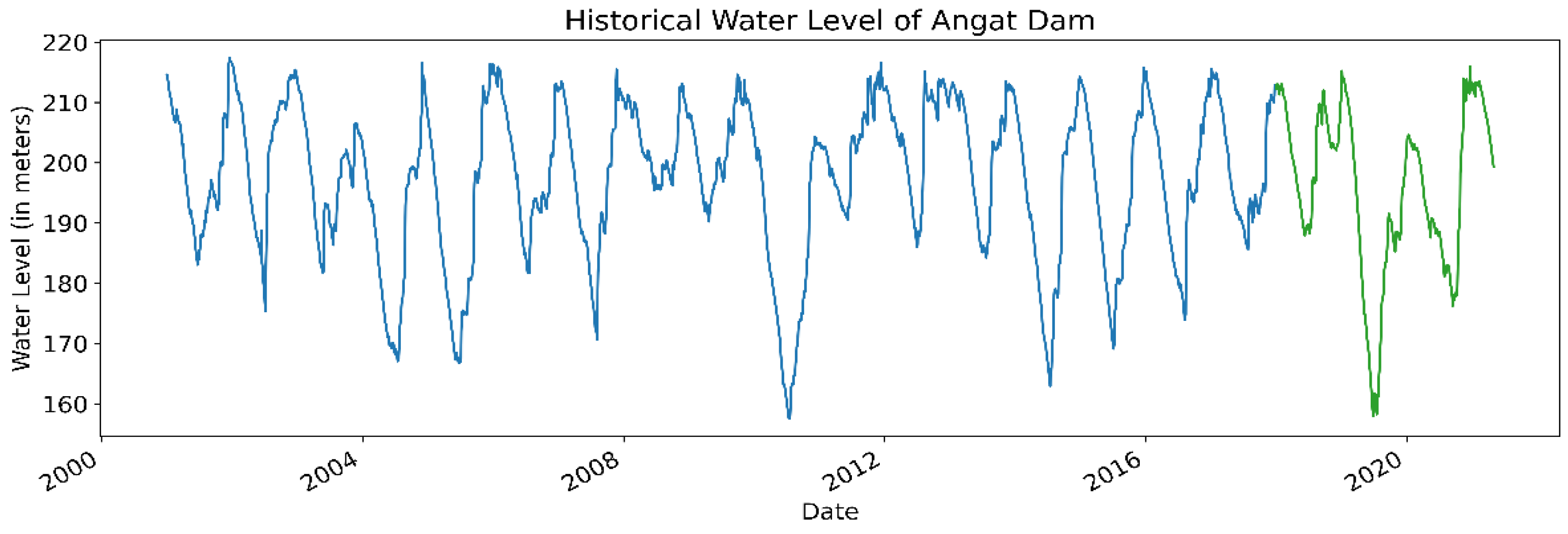
Water level data for the Angat Dam was obtained from Manila Water Company Inc. (MWCI) [20], the largest water utility firm in the Philippines and one of two concessionaires of the government-run Metropolitan Waterworks and Sewerage System (MWSS). As a concessionaire, MWCI has the right to treat, distribute, and sell the water from the Angat Dam to consumers in certain parts of Metro Manila (designated as the East Zone). The historical observations cover the period from 1 January 2001 to 30 April 2021 (over 20 years). For illustration, Figure 2 depicts the daily observations for the water level of the Angat Dam. We note that this data is publicly available, courtesy of MWSS [21].

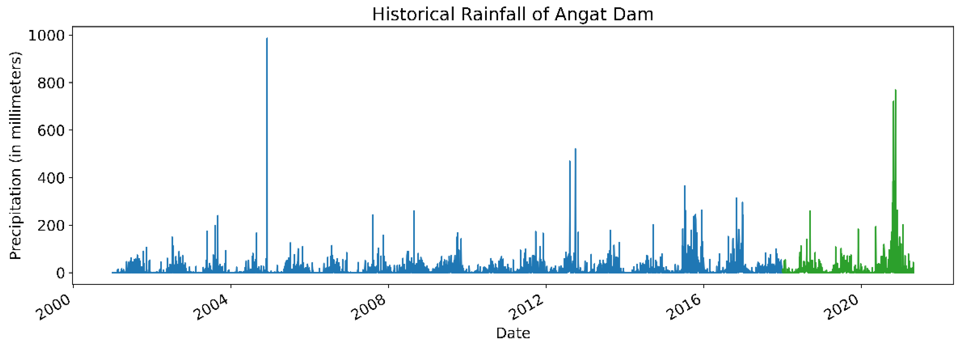
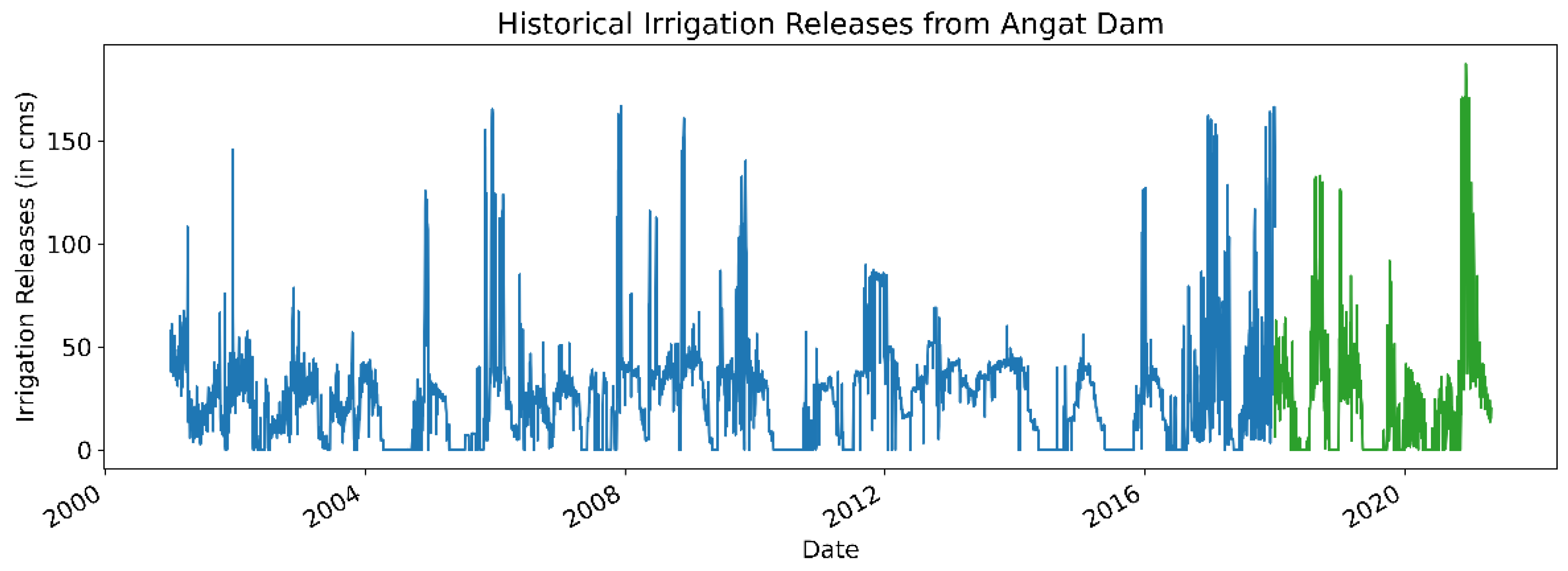
In addition to dam water levels, we examine the effects of integrating several exogenous variables on the accuracy of our forecasts. Specifically, we look at two meteorological variables (rainfall and the Oceanic Niño Index) and an irrigation variable. Figure 3, Figure 4 and Figure 5 illustrate their respective time series data, where blue observations denote the training set and green observations denote the test set. We note that since the observations of the Oceanic Niño Index (ONI) are published at a monthly level of granularity, we perform a naïve interpolation to transform the data into a daily time series. Specifically, the value for a specific month and year is used as the index’s daily observation.

In summary, the list of variables used in this study is shown in

Table 1. List of variables used in this study. All variables have a daily granularity, and the units for each are as indicated.

Variable	Units	Training Set	Test Set
Water Level	meters	1 January 2001 to 31 December 2017	1 January 2018 to 30 April 2021
Rainfall	millimeters
Oceanic Niño Index
Irrigation Releases	cubic meters per second

along with other relevant information.

2.3. Forecasting Methods

In this section we introduce the statistical and machine learning models used and describe how their parameters are tuned and selected. All methods described below are implemented in Python using the NumPy, Pandas, and Matplotlib libraries, as well as the Statsmodels, Scikit-learn, and PyTorch packages for the time series and machine learning methods.

2.3.1. Baseline Methods

To properly gauge the performance of statistical and machine learning-based forecasting methods, we opt to include the evaluation results of two simple baseline forecasting techniques: a naive method and a seasonal mean method.

The naive method constructs an n-day forecast by using the last observed value in the training set and supposing that all future values will equal that last observation,

$${\widehat{y}}_{t+n}=y_t$$

(1)

where $y_t$ is the last observed value in the data, ${\widehat{y}}_{t+n}$ are the future forecasted values, and $n$ is the number of days ahead being forecasted.

In contrast, the seasonal mean method constructs said n-day forecast by averaging all previously observed values from the same season of the year. In this case, since the data exhibits a yearly seasonality, we take the mean of the values from the same day of all previous years,

$${\widehat{y}}_{t+n}=\frac{1}{k}{\displaystyle \sum }_{i=1}^k{y}_{t+n-365\times i}$$

(2)

where $k$ is the total number of years preceding the year being forecasted. For example, to generate a 30-day forecast for 1–30 April 2019, we would calculate the average of the observations for all previous 1–30 April from 2001 to 2018 and use them as the predictions.

2.3.2. ARIMA

Autoregressive integrated moving average (ARIMA) models are a class of time series methods used to model non-stationary stochastic processes. ARIMA has been used as a benchmark for comparison against ML models, such as in [23,24,25]. The model can be broken up into three parts: An autoregressive component (AR), an integrated component (I), and a moving-average (MA) component [26].

The AR component specifies that the current value of the time series is linearly dependent on its previous values plus some error term, while the MA component specifies that the current value of the series is linearly dependent on the current and previous values of the error term,

$$y_t=c+{\displaystyle \sum }_{i=1}^p{\varphi }_i{y}_{t-i}+{\displaystyle \sum }_{i=1}^q{\theta }_i{\epsilon }_{t-i}+{\epsilon }_t$$

(3)

Finally, the I component specifies the amount of one-step differencing needed to eliminate the non-stationary behavior of the series.

Before fitting the ARIMA model, we perform pre-processing on the dataset to maximize the effectiveness of the time series model. Specifically, we transform the time series data using seasonal differencing with lag $l>1$ (not to be confused with the integrated component I whose lag $l=1$) to remove the seasonality in the data,

$$y_t=y_t-y_{t-l}$$

(4)

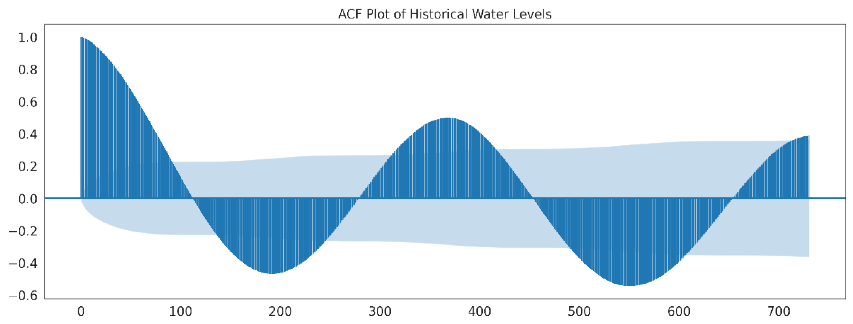
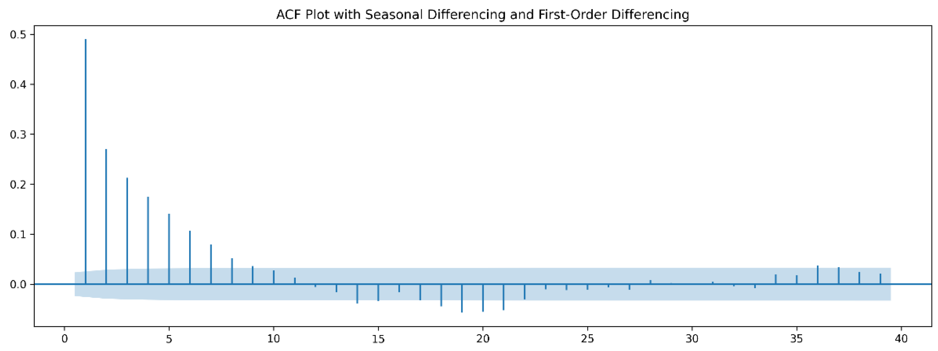
The Autocorrelation Function (ACF) plot for the Angat Dam series shown in Figure 6 indicates a one-year seasonal trend. This is illustrated by the sinusoid shape of the plot, specifically the peaks in lagged correlation that occur every 365 timesteps (in this case, days). Applying both seasonal differencing with $l=365$ and first-order differencing suppresses the seasonal trend as shown in Figure 7. For this work, we use the above differencing parameters and reverse the differencing after generating the forecasts.

We then fit an ARIMA model to the seasonally differenced series. The parameters $\left(p,d,q\right)$ are determined using a grid-search heuristic that minimizes the Akaike information criterion (AIC). AIC provides an estimate of the out-of-sample prediction error and is a commonly used statistic in the literature. The chosen model parameters are summarized in

Table 2. Summary of model parameters for the ARIMA model.

Model	Parameter	Value
ARIMA	$p$	1
	$d$	1
	$q$	2

.

To test the correctness of our estimated ARIMA model, we follow the conditions outlined by Brockwell and Davis [27] and check (1) if the data is stationary and (2) if the ACF is rapidly decreasing. We first note that the second condition is illustrated by Figure 7. Next, to check the stationarity of the differenced time series we use an Augmented Dickey-Fuller (ADF) test, which uses the model,

$$\Delta y_t=\alpha +\beta t+\gamma y_{t-1}+{\delta }_1\Delta y_{t-1}+{\delta }_2\Delta y_{t-2}+\dots$$

(5)

where $\mathsf{\Delta }$ is the first difference operator. We test the null hypothesis that $\gamma =0$ given the ADF statistic,

$$ADF=\frac{\gamma }{SE\left(\gamma \right)}$$

(6)

The test is conducted using the statsmodels.tsa package and indicates an ADF statistic of −26.76 with critical values of −3.43, −2.86, and −2.57 at 1%, 5%, and 10% significance levels, respectively. Consequently, the corresponding p-value is very close to 0. Thus, we reject the null hypothesis that the series has a unit root and conclude that the series is stationary.

We also perform a serial correlation test on the residuals using the Lljung-Box statistic,

$$Q_{LB}=n\left(n+2\right){\displaystyle \sum }_{k=1}^h\frac{{\widehat{\rho }}_k^2}{n-k}$$

(7)

and the Box-Pierce statistic,

$$Q_{BP}=n{\displaystyle \sum }_{k=1}^h{\widehat{\rho }}_k^2$$

(8)

where $n$ is the sample size, ${\widehat{\rho }}_k$ is the sample autocorrelation at lag $k$, and $h$ is the number of lags being tested. Both tests were also conducted using the previously mentioned package and reveal p values greater than 0.94 at all lags $l\le 10$, indicating that the residuals are uncorrelated. Finally, we perform a normality test using said package on the residuals using the Jarque–Bera statistic,

$$JB=\frac{n}{6}\left(S^2+\frac{1}{4}{\left(K-3\right)}^2\right)$$

(9)

where $n$ is the sample size, $S$ is the sample skewness, and $K$ is the sample kurtosis. The test results in a p value of 0.00, indicating that the residuals are non-normal. As noted in [14,27], the normality of residuals is not required for using ARIMA models. Normality as a property of the residuals merely allows us to calculate prediction intervals using analytical formulas. Since this work aims to analyze forecast accuracy and not to perform any inference on the coefficients nor to calculate confidence intervals, the non-normality of residuals should not compromise our assessment of the forecasting performance of the ARIMA model.

2.3.3. Gradient Boosting Machines

Boosting methods are a type of ensemble method that combines several base models to produce a single optimal predictive model. Compared to conventional techniques, optimization in boosting is done in a parametrized function space, which can be extended to parametrized base-learner functions [28].

In this work, we use gradient boosting machines (GBM), a class of boosted models that utilizes gradient descent to minimize the differentiable loss function of a model by iteratively optimizing “weak learners” (usually simple models with relatively low predictive power) that concentrate on areas where the existing learners are performing poorly. Note that while any model can be used, the method is typically associated with decision trees, which we use in this study. Tree-based implementations of GBM are defined by several parameters such as the learning rate (which controls the gradient update steps), max depth (the maximum depth of a tree), and $n$ estimators (the number of trees/boosting stages).

The algorithm works as follows: First, it begins by computing an initial estimate of the target variable based on the average value. Second, the residuals are calculated using the initial estimates and the actual observed values. Third, a tree model, whose depth is controlled by the max depth parameter, is trained to predict these residuals. Fourth, the new estimate is given by a combination of the old estimate and the forecasted residuals. In order to prevent overshooting, the forecasted residual is modulated by the learning rate parameter. Finally, the algorithm returns to the second step and is repeated up to a desired number of stages, which is controlled by the $n$ estimators parameter.

Mathematically, if we wish to train an ensemble model $f\left(x\right)$ to predict $y$, then GBM constructs the ensemble model at each stage $m=1,2,\dots ,n$ estimators such that,

$$f_{m+1}\left(x\right)=f_m\left(x\right)+\alpha h_m\left(x\right)$$

(10)

where $\alpha$ is the learning rate and given a squared error loss function,

$$L=\frac{1}{2}{\left(y-f\left(x\right)\right)}^2$$

(11)

the new estimator $h_m\left(x\right)$ is given by:

$$h_m\left(x\right)=-\frac{\partial L}{\partial f_m}=y-f_m\left(x\right)$$

(12)

Several works have evaluated the use of GBM as a time series forecasting model, such as in [29,30,31]. GBM and its variants have been a popular choice of model in the recently concluded M5 Competition and many other time series forecasting competitions where they have been demonstrated to provide the most robust results that balance accuracy and training time [16].

Due to their non-linear nature, GBM models can learn the complex seasonal features of the data. In addition, GBMs can handle multiple predictor variables. Thus, data for the dam water levels, rainfall, irrigation releases, and ONI were used as input variables for our implementation of GBM.

Since we are using a machine learning regression model on time series data, we must first decide on an appropriate lookback window (i.e., the number of days we lookback to predict the future). This is equivalent to the $p$ parameter of an AR process. For this study, we heuristically select the window size to be double the length of the forecast horizon, except in the case of the 1-day-ahead forecast where we choose a 7-day lookback window. Based on plots of the water level series and its ACF plots, we observe that the window sizes of the lookbacks give sufficient opportunity for the trends and seasonality of the time series to emerge, given the length of the target horizon.

When choosing the hyperparameters for our GBM models, we again use a grid-search heuristic and select the parameters that minimize the mean absolute error (MAE). The chosen model parameters are summarized in

Table 3. Summary of model parameters for the GBM model.

Model	Forecast Horizon	Window Size	Parameters	Value
GBM (Multivariate)	1	7	loss	least squares
	30	60	learning rate	0.1
	90	180	max depth	5
	180	365	n estimators	50

.

2.3.4. Deep Neural Networks

Neural networks (NN) are a family of machine learning models that attempt to mimic the structure of the biological brain. NNs have been applied to a wide variety of time series forecasting problems in a meteorological context, such as weather forecasting [32,33,34] and solar radiation modeling [35,36]. Like GBMs, they can handle multiple independent variables and learn the non-linear relationships between these input variables. In this work, we focus our attention on deep neural networks (DNN), which are models characterized by many deep hidden layers (often with complex architectures) capable of learning efficient representations of high-dimensional data. We use the long short-term memory (LSTM), a type of recurrent neural network (RNN) that is designed to handle sequential data such as text data and time series data [37].

Compared to a standard RNN, LSTMs have a similar recurrent feedback structure, however they have additional components that can regulate the flow of information at each time step. Essentially, these regulating components allow the architecture to better deal with the vanishing gradient problem (i.e., multiplying many small gradients can cause the gradient updates to go to zero) that RNNs sometimes experience during training. For illustration, Figure 8 depicts the internal structure of an LSTM cell. From left to right, the $\sigma$-blocks are called the forget $f$, input $i$, and output gates $o$, respectively. The forget gate controls the amount of information being let through from the previous cell state $c_{t-1}$. The input gate is used to determine the new cell state $c_t$ given the current input $x_t$ and previous hidden state $h_{t-1}$. Furthermore, the output gate is used to determine the new hidden state $h_t$. Formally, the gate and state Equations of each component are given by:

$$f_t=\sigma \left(W_{if}{x}_t+b_{if}+W_{hf}{h}_{t-1}+b_{hf}\right)$$

(13)

$$i_t=\sigma \left(W_{ii}{x}_t+b_{ii}+W_{hi}{h}_{t-1}+b_{hi}\right)$$

(14)

$$o_t=\sigma \left(W_{io}{x}_t+b_{io}+W_{ho}{h}_{t-1}+b_{ho}\right)$$

(15)

$$c_t=f_t⨀c_{t-1}+i_t⨀tanh\left(W_{ic}{x}_t+b_{ic}+W_{hc}{h}_{t-1}+b_{hc}\right)$$

(16)

$$h_t=o_t⨀tanh\left(c_t\right)$$

(17)

where $\sigma$ refers to a sigmoid activation function and $⨀$ refers to an element-wise product operator.

In this paper, we examine two versions of the DNN model: a univariate LSTM-based encoder-decoder model (DNN-U) that only uses lagged water levels as input and a multivariate model (DNN-M) that incorporates the exogenous variables discussed above, together with the historical water levels.

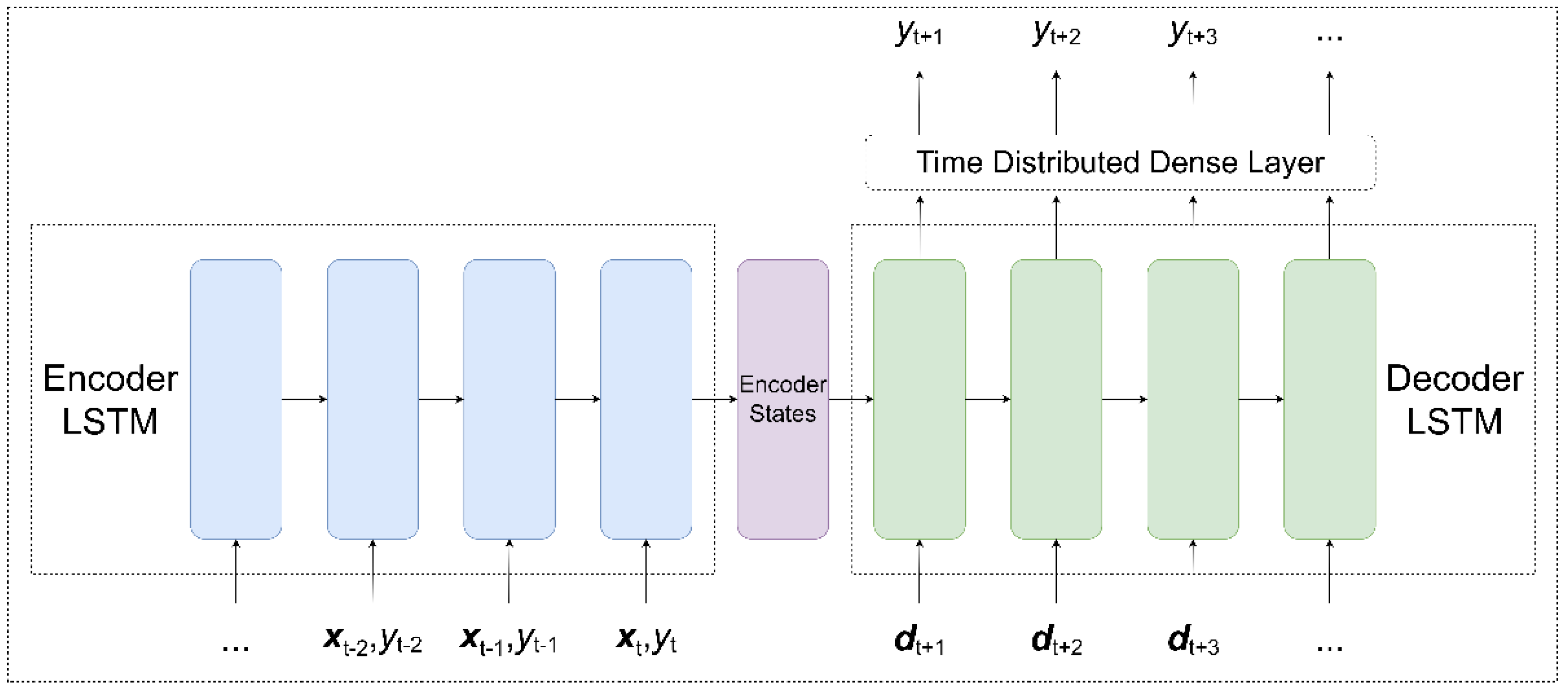
Our DNN models closely follow the original sequence-to-sequence (seq2seq) architecture proposed by Sutskever et al. [38]. As illustrated in Figure 9, the encoder LSTM takes in lagged observations of the water level $y$ and exogenous variables $x$ (which are absent in DNN-U) and encodes them into a hidden state $h$ and cell state $c$. These encoder states are then used as the initial states for the decoder LSTM, which accepts known future dates $d$ as input, representing the target dates we wish to forecast. The decoder outputs are then passed to a time distributed dense layer, which generates the actual forecasts.

For the decoder inputs, each month–day date is encoded into a pair of features $d_t=\left[d_{sin},d_{cos} \right]$ using sine and cosine transformations (called trigonometric or cyclical encoding),

$$d_{sin}=sin\left(\frac{z_t}{365}\times 2\pi \right)$$

(18)

$$d_{cos}=cos\left(\frac{z_t}{365}\times 2\pi \right)$$

(19)

where $z_t=0,1,2,\dots$ is an index variable corresponding to the date at time $t$. This specific encoding allows us to represent the 365-day periodicity of the dates as a pair of values each between −1 and 1.

This particular DNN architecture possesses several advantages. First, the model provides a way to incorporate known future exogenous variables if they are available. Second, the LSTM-based encoder can accept a variable length input at the inference time. This implies that one does not have to input the entire history to make predictions, which is more convenient for shorter horizons. Third, the LSTM-based decoder allows us to produce forecasts of arbitrary length. This means that we can train a single model to generate multi-horizon forecasts. For the window size, we set this to 365 since water levels exhibit a 365-day seasonality. For the number of LSTM units, we perform a grid-search heuristic on the set {8, 16, 32, 64, 128} and select the parameter that minimizes MAE. For the sake of tractability, the other training parameters and hyperparameters for the DNN models were kept on their default settings or manually tuned. The chosen model parameters are summarized in

Table 4. Summary of model parameters for the DNN-U and DNN-M model.

Model	Forecast Horizon	Window Size	LSTM Units	Parameters	Value
DNN-U (Univariate)	1	365	64	activation	tanh
	30			epochs	50
DNN-M (Multivariate)	90			batch size optimizer	63 Adam
	180			loss	Huber

.

2.4. One-Step and Multi-Step Forecasting

In this work, both one-step and multi-step forecasting of daily dam levels are attempted. A one-step forecast describes the prediction of a future event that is one-step ahead of the last observed value in a time series. Similarly, an $n$-step forecast predicts $n$ sequential future events (i.e., $n$-step ahead of the last observation). This work examines the performance of our models in generating 1-day, 30-day, 90-day, and 180-day forecasts. We believe that these prediction horizons should capture short-term and long-term forecasting scenarios that may arise in water resource management problems. In practice, our proposed architecture is able to predict any arbitrary horizon length.

2.5. Evaluating Model Performance

To evaluate model performance, we use three error metrics: mean absolute error (MAE), root mean squared error (RMSE), and mean absolute percentage error (MAPE). We also include the R² statistic as a goodness-of-fit measure. These are defined as,

$$MAE=\frac{1}{n}{\displaystyle \sum }_{i=1}^n\left|y_i-{\widehat{y}}_i\right|$$

(20)

$$RMSE=\sqrt{ \frac{1}{n}{\displaystyle \sum }_{i=1}^n{\left(y_i-{\widehat{y}}_i\right)}^2}$$

(21)

$$MAPE=100\times \frac{1}{n}{\displaystyle \sum }_{i=1}^n\left|\frac{y_i-{\widehat{y}}_i}{y_i}\right|\%$$

(22)

$$R^2=1-\frac{{{\displaystyle \sum }}_{i=1}^n{\left(y_i-{\widehat{y}}_i\right)}^2}{{{\displaystyle \sum }}_{i=1}^n{\left(y_i-\overline{y}\right)}^2}$$

(23)

where $y_i$ is the true value, ${\widehat{y}}_i$ is the forecasted value, $\overline{y}$ is the mean of the observed data, and $n$ is the number of data points being forecasted.

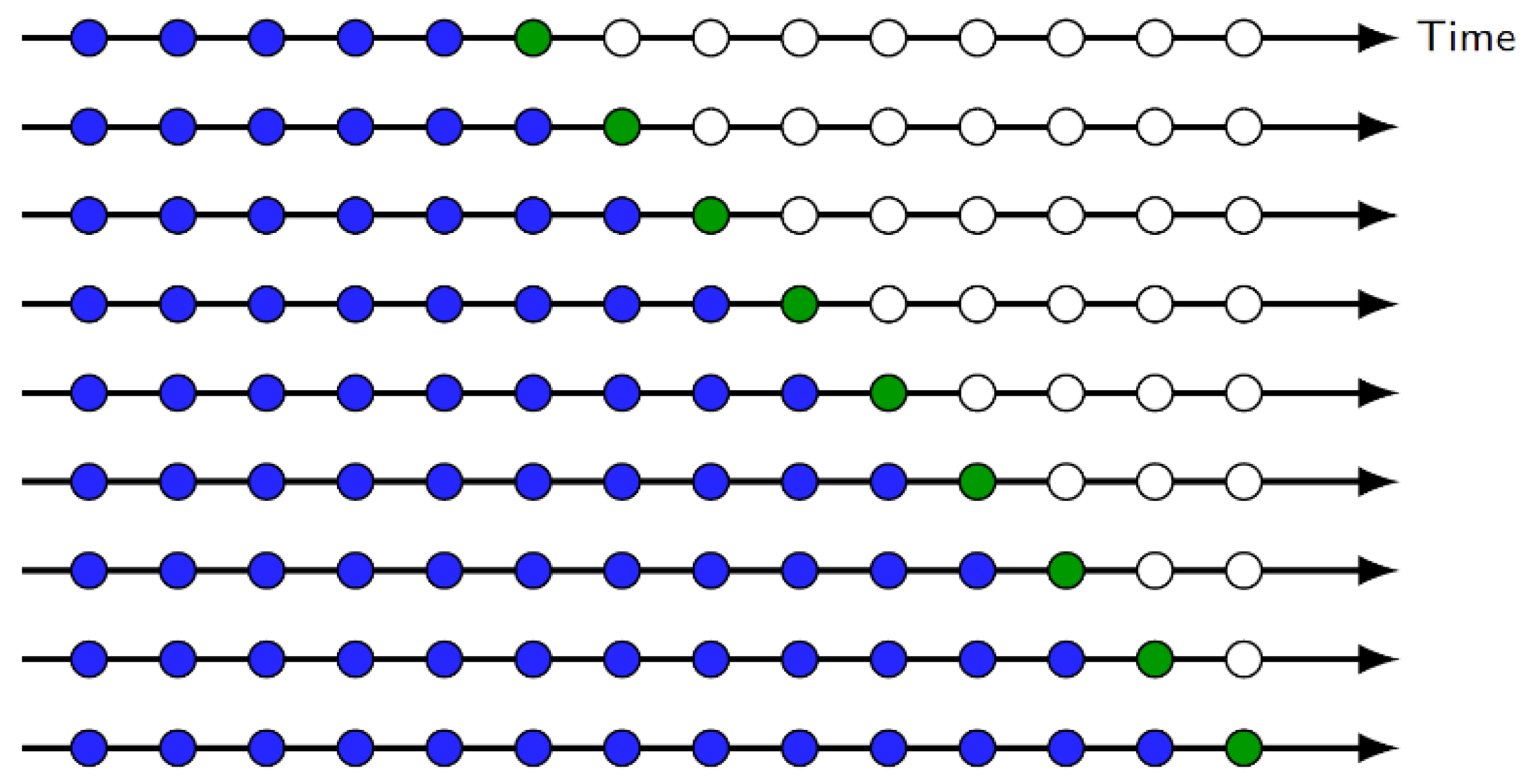
In addition, this work proposes the use of time series cross-validation (TSCV). Cross-validation is a resampling technique typically used in prediction problems to gain insight into how well a model generalizes and as a method for estimating the uncertainty of error statistics. For time series data, using standard cross-validation methods (e.g., k-fold cross-validation) is inappropriate due to the sequential nature of the data. Thus, TSCV is used to produce unbiased estimates of the error statistics. In this procedure, the distribution of the error metric (e.g., MAE, RMSE, MAPE) is estimated by calculating the statistic over a series of test sets.

As an example, Figure 10 illustrates this process for one-step-ahead forecasting. After calculating the error metric, we serially construct training and test partitions by “rolling in” test observations. Note that the training set consists only of data that occurred prior to the observations that form the test set. Thus, no future observations can be used in constructing the forecast, leading to an unbiased estimate. The process is similar for an $n$-day-ahead forecast, with the test set containing n observations instead of one.

For training and testing, the setup is as follows: the last 1215 data points (i.e., observations from 1 January 2018 to 30 April 2021) are withheld as the initial test set and the remaining observations comprise the initial training set. After training a model and calculating the test metrics, the next day’s observation is removed from the test set and rolled into the training set. The process is repeated until the test set is exhausted, and we have constructed an approximation for the test metric’s sampling distribution. We then calculate the average and standard deviations of the error statistics to summarize model performances.

3. Results and Discussion

3.1. Time Series Description and Characteristics

Before discussing model performance, we briefly describe some notable characteristics of our time series datasets.

For daily rainfall, we note that spikes in the dataset (seen in Figure 3) can be attributed to periods of intense rain usually caused by the monsoon season or typhoons. For example, the massive spike in rainfall at the tail end of 2004 corresponds to the passage of Typhoon Nanmadol through Luzon Island [39].

Next, we incorporate climate data through the Oceanic Niño Index. This is one of the main indices used to track the El Niño-Southern Oscillation (ENSO), a climate phenomenon that affects temperature and precipitation worldwide. Since dam levels are primarily driven by rainfall, and rainfall is heavily influenced by the El Niño and La Niña phenomena, we believe that the addition of ONI should help with our forecasting models.

Lastly, a portion of the water stored in the Angat Dam is allocated for farmland irrigation. Consequently, there is a strong relation between irrigation releases and daily water levels. The irrigation releases are scheduled by the National Irrigation Administration (NIA), a government-owned and controlled corporation responsible for irrigation development and management.

3.2. Model Performance Results and Analysis

We now discuss and summarize the performance of each forecasting model.

Table 5. Estimates for MAE, RMSE, MAPE, and R² calculated using TSCV for a 1-day forecast.

1-Day Forecast
Model	MAE	RMSE	MAPE	R2
Naïve	0.291 (0.424)	0.291 (0.424)	0.002 (0.002)	0.999
Seasonal Mean	8.088 (6.080)	8.088 (6.080)	0.043 (0.036)	0.560
ARIMA	0.261 (0.467)	0.261 (0.467)	0.001 (0.002)	0.999
GBM	0.256 (0.411)	0.256 (0.411)	0.001 (0.001)	0.999
DNN-U	0.198 (0.390)	0.198 (0.390)	0.001 (0.002)	0.999
DNN-M	0.239 (0.372)	0.239 (0.372)	0.001 (0.002)	0.999

,

Table 6. Estimates for MAE, RMSE, MAPE, and R² calculated using TSCV for a 30-day forecast.

30-Day Forecast
Model	MAE	RMSE	MAPE	R2
Naïve	3.344 (2.631)	3.909 (2.991)	0.017 (0.014)	0.890
Seasonal Mean	8.136 (5.818)	8.371 (5.795)	0.043 (0.034)	0.560
ARIMA	3.379 (2.732)	4.008 (3.148)	0.017 (0.014)	0.896
GBM	3.059 (2.501)	4.557 (2.818)	0.016 (0.005)	0.890
DNN-U	2.938 (2.368)	3.322 (2.576)	0.015 (0.013)	0.906
DNN-M	2.892 (2.263)	3.273 (2.493)	0.015 (0.013)	0.910

,

Table 7. Estimates for MAE, RMSE, MAPE, and R² calculated using TSCV for a 90-day forecast.

90-Day Forecast
Model	MAE	RMSE	MAPE	R2
Naïve	8.390 (5.469)	9.825 (6.157)	0.044 (0.029)	0.358
Seasonal Mean	8.210 (4.954)	8.987 (5.069)	0.044 (0.030)	0.565
ARIMA	7.934 (5.287)	9.339 (6.021)	0.041 (0.028)	0.411
GBM	6.209 (3.603)	8.261 (3.989)	0.033 (0.006)	0.638
DNN-U	5.371 (2.965)	6.243 (3.312)	0.028 (0.016)	0.735
DNN-M	5.103 (3.091)	5.962 (3.510)	0.027 (0.017)	0.746

and

Table 8. Estimates for MAE, RMSE, MAPE, and R² calculated using TSCV for a 180-day forecast.

180-Day Forecast
Model	MAE	RMSE	MAPE	R2
Naïve	13.408 (7.079)	15.475 (7.856)	0.070 (0.040)	−0.702
Seasonal Mean	8.469 (3.791)	9.911 (3.845)	0.046 (0.023)	0.472
ARIMA	11.431 (4.947)	13.614 (5.422)	0.060 (0.026)	−0.360
GBM	7.335 (2.743)	9.578 (3.109)	0.039 (0.005)	0.518
DNN-U	7.113 (2.982)	8.668 (3.445)	0.038 (0.018)	0.547
DNN-M	6.652 (3.092)	8.128 (3.767)	0.036 (0.019)	0.581

show the average MAE, RMSE, and MAPE estimates with their standard deviations, indicating the accuracy of the predictions and the associated uncertainty for each metric, respectively. For completeness, we also include the R² statistics, which illustrates the goodness-of-fit of the models for each prediction horizon. In the discussions below, we focus our attention on the MAE, RMSE, and MAPE metrics as these statistics more appropriately measure prediction accuracy and how well the model generalizes any unseen (i.e., future) data.

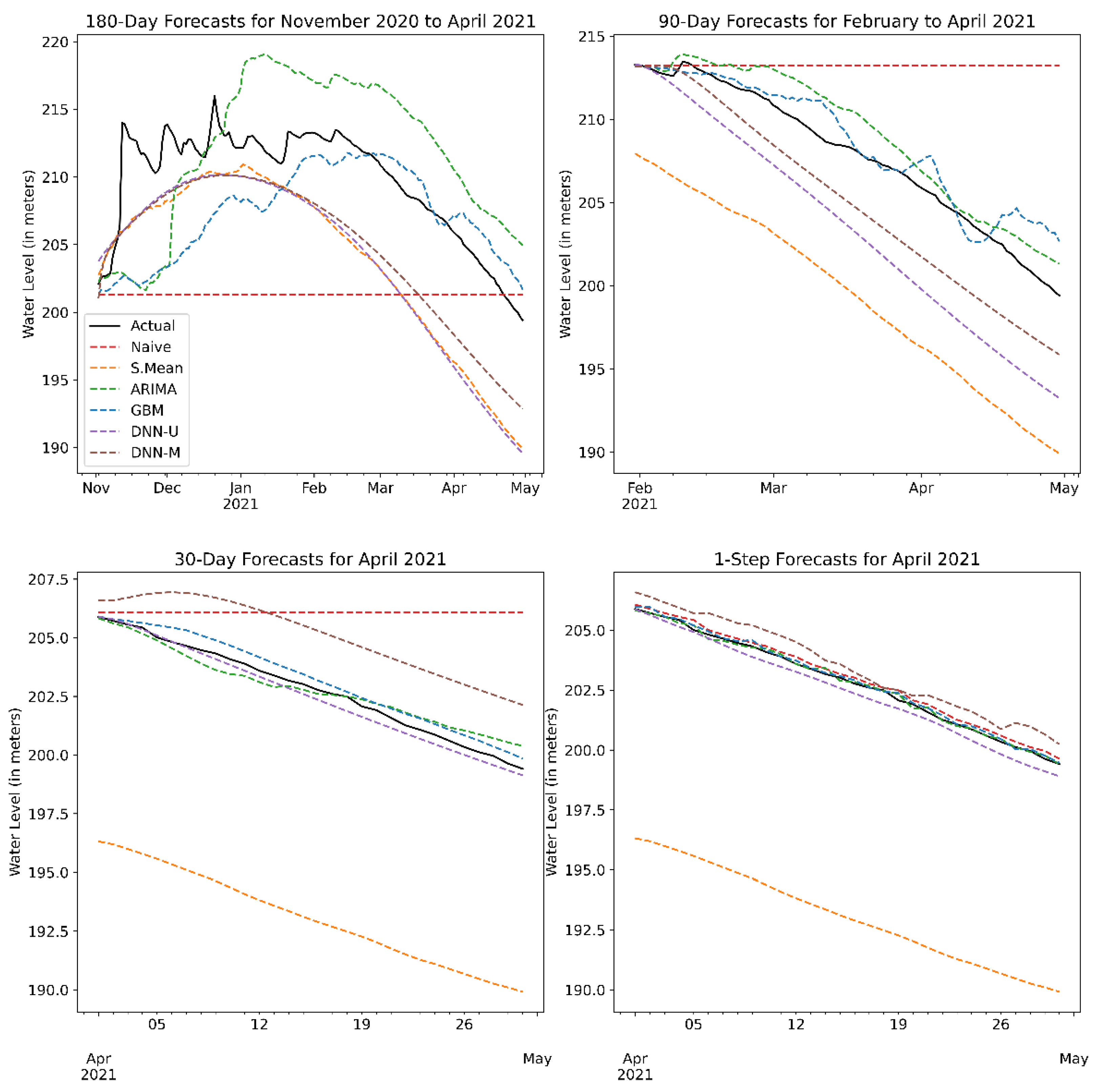
Figure 11 depicts a snapshot of sample forecasts for each of the forecasting methods at each prediction horizon. We note that the naïve and seasonal mean methods are meant to be baselines for the short-term and long-term horizons, respectively. Hence, their noticeably poor performance at the opposing extreme horizons. The sample forecasts are purely meant to be illustrative, as each forecast only represents a single test set in the time series cross-validation. As such, the plots do not represent the average performance of each method.

Overall, our results show that the statistical and ML models had lower errors on average and higher goodness-of-fit scores compared to the naïve and seasonal mean methods. In particular, the non-parametric ML models showed superior performance compared to the linear ARIMA model, with both DNNs having the more accurate water level forecast (across all metrics) for both short- and long-term horizons with the least amount of uncertainty.

For 1-day-ahead forecasting, the best performing model, DNN-U, displayed a 32% improvement in MAE/RMSE over the baseline naïve/persistence forecast. This result highlights how much additional performance is gained, given the relative complexity and intensive computational requirements of deep neural networks versus a naïve method that is calculated effortlessly. Essentially, this allows us to properly contextualize the trade-off between the model’s complexity and its performance. In this scenario, it appears that a univariate model (i.e., no exogenous predictors) has superior performance when compared to its multivariate counterparts. This result seems to imply that for very short horizons, the addition of covariates is actually detrimental to performance. From a practical perspective, fewer variables mean it becomes easier for the model to learn and less computational power is needed.

In the 30-day horizon, we see that the DNN-M slightly edges out its univariate counterpart. This suggests that recent observations of rainfall and the climate index (which influences dam inflow) together with irrigation releases (a primary driver of outflow) possesses information that the neural network can learn from.

We see this trend continue for long-term forecasts, where the multivariate DNN model takes the clear lead in terms of all error metrics. For the 90-day-ahead forecast, DNN-M displayed a 0.27 m and a 0.28 m improvement over DNN-U’s MAE and RMSE scores, respectively. This also applies to the 180-day-ahead forecasts, with DNN-M showing lower average MAE, RMSE, and MAPE scores, as well as having less uncertainty in regard to the estimates. Of particular note is the fact that DNN-M exhibits a 21% improvement in MAE and an 18% improvement in RMSE, over a baseline seasonal mean forecast. Effectively, this measures how much more effective the DNN-M model is over simply taking the average water level of previous years. These results highlight and quantify the effect of exogenous variables on forecast accuracy and its uncertainty. In this case, adding predictors can lead to a higher number of errors in very short-term forecasts, however leads to better performance once we start generating predictions with longer horizons.

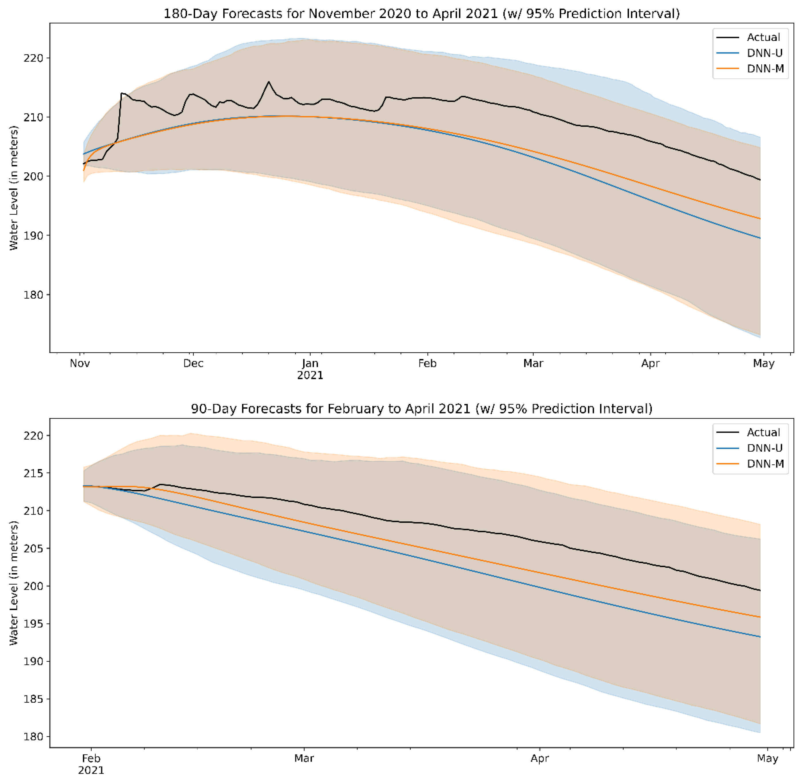
In addition to examining point forecasts, one can also look at prediction intervals in order to gauge the uncertainty around the predictions themselves. Figure 12 presents a sample forecast for two long-term scenarios: a 6-month forecast covering November 2020 to April 2021 and a 3-month forecast covering February to April 2021. As DNNs are inherently non-probabilistic in nature, calculating a prediction interval in an analytical fashion is not possible. Thus, we apply a bootstrapping method on the model’s residuals in order to estimate the prediction intervals [14].

As the plots illustrate, the uncertainty around our predictions increases the further ahead we try to forecast. In the case of the 3-month forecast, the DNN-U appears less optimistic about the water level in the coming months, as its prediction bands diverge slightly from those of its multivariate counterpart. The DNN-M model’s slight uptrend looks more accurate however, given the slight bump in water level observed at the middle of February. For the 6-month forecast, it appears that the multivariate DNN model has a tighter band compared to DNN-U, especially in the period after February, corresponding to the summer season in the Philippines. This suggests that conditioning our forecasts on historical climate, rainfall, and irrigation trends can lessen the uncertainty of a long-term prediction, especially at critical times of the year when rainfall is sparse.

3.3. Effects of Exogenous Variables on Multi-Step Forecasting Performance

In this section, we analyze the effects of each exogenous variable on the multi-step prediction accuracy of our DNN model. Previously, we have seen that the DNN-M, which uses all available exogenous variables, outperforms the DNN-U in the multi-step forecasting, especially in the longer-term horizons. We are interested in understanding if some of these variables actually impede performance, which may run contrary to intuition.

Table 9. Average estimates for MAE and RMSE, and their standard deviations calculated using TSCV for a 180-day forecast across different combinations of exogenous variables.

180-Day Forecast (DNN)
Exog. Variables	MAE	RMSE
Rain, Irrigation, ONI	6.652 (3.092)	8.128 (3.767)
Rain, Irrigation	6.458 (3.432)	7.997 (4.003)
Rain, ONI	6.739 (3.479)	8.290 (4.213)
Irrigation, ONI	7.040 (2.708)	8.523 (3.341)
Rain	6.601 (3.352)	8.142 (3.942)
Irrigation	6.551 (3.248)	7.999 (3.827)
ONI	6.814 (2.450)	8.258 (3.025)
No Exog.	7.113 (2.982)	8.668 (3.445)

,

Table 10. Average estimates for MAE and RMSE, and their standard deviations calculated using TSCV for a 90-day forecast across different combinations of exogenous variables.

90-Day Forecast (DNN)
Exog. Variables	MAE	RMSE
Rain, Irrigation, ONI	5.103 (3.091)	5.962 (3.510)
Rain, Irrigation	5.034 (3.317)	5.870 (3.729)
Rain, ONI	5.146 (3.393)	5.986 (3.812)
Irrigation, ONI	5.367 (2.869)	6.225 (3.216)
Rain	5.108 (3.278)	5.960 (3.698)
Irrigation	5.370 (3.022)	6.223 (3.479)
ONI	5.375 (2.773)	6.272 (3.114)
No Exog.	5.371 (2.965)	6.243 (3.312)

and

Table 11. Average estimates for MAE and RMSE, and their standard deviations calculated using TSCV for a 30-day forecast across different combinations of exogenous variables.

30-Day Forecast (DNN)
Exog. Variables	MAE	RMSE
Rain, Irrigation, ONI	2.892 (2.263)	3.273 (2.493)
Rain, Irrigation	2.880 (2.512)	3.253 (2.692)
Rain, ONI	2.953 (2.437)	3.321 (2.632)
Irrigation, ONI	3.039 (2.375)	3.398 (2.588)
Rain	2.763 (2.283)	3.160 (2.516)
Irrigation	2.901 (2.249)	3.315 (2.486)
ONI	2.942 (2.318)	3.338 (2.543)
No Exog.	2.938 (2.368)	3.322 (2.576)

summarize the average MAE and RMSE values for every possible combination of exogenous variable. We note that the differences in the MAPE and R² values were very minimal across the combinations. As such, we omit them from our results.

In the 180-day and 90-day forecast horizons, we see that the combination of rainfall and irrigation gives results that are superior to using all available variables. In the 30-day horizon, using only the rainfall variable gave the best accuracy. In fact, our results suggest combinations that don’t include the climate variable, represented by the Oceanic Niño Index, have lower average MAE and RMSE scores. While a more sophisticated causal analysis of the relationship between each covariate is beyond the scope of this work, we can see that naively adding features to the DNN model can have negative empirical effects on the quality of the forecasts.

3.4. Practical Implications

In terms of practical application, our methodology can be used to evaluate multiple water level forecasting models. Ultimately, well-performing models can be selected by water resource managers for long-term strategic planning and short-term intervention. A common use case described by the domain experts of the operations and planning team of MWCI is scenario planning. This is when they consider several dam level scenarios and prepare allocation and conservation strategies for each situation. Water utility companies that provide drinking water and wastewater services in the Philippines typically need a 6-month ahead (180-day ahead) forecast at minimum to properly plan contingency measures for the following summer season when water levels are at their lowest.

For short-term use cases, 1-day ahead forecasts are not as critical to the day-to-day operations of a water utility, although this tends to be the focus of most of the works described previously. Instead, operations and planning managers favor periods within the range of 1-week and 1-month ahead forecasts as these horizons allow them ample time to plan and execute short-term interventions. These interventions include dam operators scheduling ad hoc water releases during periods of strong rainfall brought about by typhoons due to immediate threats to the structural integrity of a dam. Naturally, the proper planning of these types of occurrences can have an impact beyond the water industry, as situations like those described earlier can be tied to external events such as the flood disaster risk management of nearby areas.

As a regulated industry, having high quality forecasts that are both data-driven and rigorously validated can significantly reduce the uncertainty faced by water utilities and, at the same time, increase transparency for regulators by having a precise and formalized methodology.

4. Conclusions

This work has proposed a comprehensive framework for evaluating water level forecasts that addresses several significant gaps in the methodologies of previous studies. We have evaluated the performance of several statistical and machine learning-based forecasting methods in predicting the daily water levels of the Angat Dam. Our results indicate that DNN models outperform classic models like ARIMA and other machine learning models like GBM. This is in terms of average MAE, RMSE, and MAPE values estimated using a time series cross-validation approach. Both GBM and DNN models also tended to have a lower level of uncertainty in regard to the MAE, RMSE, and MAPE estimates compared to the baseline methods.

Additionally, the DNN-U variant showed superior performance in generating 1-day forecasts when compared to its multivariate counterpart. This indicates that naïvely adding exogenous predictors to a forecasting method does not necessarily lead to better performance, and in fact, it may lead to more difficulties in training ML models, as more noise is added to the system. However, for multi-step forecasting, especially long-term forecasting, we see that the DNN-M shows better performance, beating out both GBM and DNN-U. This indicates that deep neural networks can incorporate multiple variables that exhibit complex behavior to produce superior forecasts with long time horizons. However, our results also show that certain combinations of covariates can still have a negative impact on forecast accuracy. Thus, careful analysis of the relationship between the target variable and each exogenous variable is critical in order to train robust forecasting models.

While the results shown in this study have been focused on the Angat Dam, the methodologies described here can be applied to other forecasting problems in water resource management and hydrological research. Recent studies have shown how powerful deep neural networks (and machine learning in general) are at learning complex patterns in time series data. Our work demonstrates that much of the work in the literature can be improved on, not just in terms of model complexity but also in designing a more robust evaluation methodology for one-step and multi-step forecasting scenarios by using resampling techniques such as time series cross-validation.

For future work, deeper analysis of explanatory and exogenous variables is recommended. Feature importance analysis of machine learning models and explainable AI is a new and developing field of research that can help identify and quantify which variables provide measurable and significant gains to predictive performance. Formal techniques in causal analysis can also be applied to the relevant covariates to determine if these variables truly warrant inclusion in the modeling process. Additionally, a more thorough and empirical examination of lookback window sizes and other hyperparameters can be conducted to further optimize the performance of ML and DL models. This includes optimizations to the DNN architectures and its various training parameters. In particular, a more detailed ablation study of the various DNN components that explores their strengths and weaknesses can be made. Finally, an ideal forecasting method should also be able to incorporate future dam release decisions made by management and regulators. Thus, scenario-based modeling techniques that incorporate the expert judgement of dam managers and regulators can also help improve the usability of said methods.