
Spiking Neural Networks for Computational Intelligence: An Overview


1
Department of Computer Science, Loughborough University, Loughborough LE11 3TU, UK
2
Intelligent Systems Research Centre, Ulster University Magee Campus, Derry BT48 7JL, UK
3
Knowledge Engineering and Discovery Research Institute, Auckland University of Technology, Auckland 1010, New Zealand
*
Author to whom correspondence should be addressed.
Big Data Cogn. Comput. 2021, 5(4), 67; https://doi.org/10.3390/bdcc5040067
Submission received: 26 September 2021
/
Revised: 3 November 2021
/
Accepted: 9 November 2021
/
Published: 15 November 2021
(This article belongs to the Special Issue Computational Intelligence: Spiking Neural Networks)
Abstract
:Deep neural networks with rate-based neurons have exhibited tremendous progress in the last decade. However, the same level of progress has not been observed in research on spiking neural networks (SNN), despite their capability to handle temporal data, energy-efficiency and low latency. This could be because the benchmarking techniques for SNNs are based on the methods used for evaluating deep neural networks, which do not provide a clear evaluation of the capabilities of SNNs. Particularly, the benchmarking of SNN approaches with regards to energy efficiency and latency requires realization in suitable hardware, which imposes additional temporal and resource constraints upon ongoing projects. This review aims to provide an overview of the current real-world applications of SNNs and identifies steps to accelerate research involving SNNs in the future.
1. Introduction
Similar to artificial neural networks (ANN), spiking neural networks (SNN) are also inspired by the neural networks observed in biology. However, unlike ANNs, SNNs employ processing units that process information using neuronal units that are much closer to their biological counterparts. Biological neurons process and transmit information using action potentials, also known as spikes, which underlie the incredible energy efficiency exhibited by the brain. These similarities between spiking neurons and biological neurons also imply that SNNs with similar power requirements as the human brain could potentially be developed. This has motivated several studies to compare ANNs and SNNs from different perspectives [1,2,3]. Despite these capabilities, SNNs have not seen the same level of advances as observed in ANNs.
In this review article, we present recent advances in the development of technical approaches for learning in SNNs and their real-world applications. The ideas discussed in the next seven sections can be used to identify important areas for current and future research on SNNs that could potentially close the gap between ANNs and SNNs. The layout of this article is as follows: Section 2 describes the fundamental principles underlying a spiking neuron. Section 3 presents different architectures of SNNs that have been developed using spiking neurons. Section 4 provides an overview of different learning algorithms that have been proposed for training SNNs. Generic applications of SNNs are presented in Section 5. Section 6 presents the development of neuromorphic hardware systems for SNN. Section 7 presents one trend in the development of SNN architectures called brain-inspired SNN, along with their specific applications. Section 8 is the conclusion for this review and offers a discussion.
2. Fundamentals of a Spiking Neuron
The fundamental units that process information in spiking neural networks are called spiking neurons. Inspired by biological neurons, spiking neurons utilize temporal signals consisting of binary events, termed as spikes, as their input and output. Spiking neurons utilize the precise time of spikes to encode information. Each spike received by a spiking neuron alters its state, which is termed as membrane potential. When the membrane potential of a neuron reaches a certain threshold value, the spiking neuron generates a spike that is transmitted to other spiking neurons over a synapse.
The response of a biological neuron depends on a multitude of ionic currents inside and outside the cell membrane. Hodgkin and Huxley proposed a detailed computational model based on the information propagation in a giant axon of the squid [4]. However, a detailed computational model of a biological neuron is less suitable for applications in computational intelligence because of its excessive computational overhead. To overcome this issue, several computationally efficient spiking neuron models have been proposed in literature, such as the leaky integrate-and-fire (LIF) neuron [5] and Izhikevich neuron [6]. Below, we provide a description of the LIF neuron and Izhikevich neuron for discussing the topics presented in subsequent sections. A thorough discussion on various existing spiking neuron models has been presented in [7].
2.1. Leaky Integrate-and-Fire Neuron
The membrane potential () at time of an LIF neuron is described by the following differential equation
where represents the membrane potential of the neuron at time , and represents the resting potential, i.e., the potential of the neuron when it is not receiving any input. represents the time constant of the neuron and represents the resistance of the neuron. represents the input current received by the neuron over the incoming synapses.
2.2. Izhikevich Neuron Model
The Izhikevich neuron [6] was developed with the aim of reproducing the spiking characteristics of various cortical neurons using a computationally simple model. The membrane potential () and membrane recovery variable () of a spiking neuron modeled as an Izhikevich neuron are given by
provides negative feedback to , thereby making it harder for a neuron to spike again after generating a spike. The neuron generates a spike when its potential crosses a threshold value (). After every spike, the value of is reset to the resting potential and the value of is incremented by . In Equation 3, the parameter determines the time scale of and the parameter captures the impact of subthreshold variations in on . Together, the values for the parameters , , and in the above equations enable simulation of different spiking behaviors exhibited by cortical neurons.
3. Architectures of Spiking Neural Networks
There are primarily two types of architectures that have been utilized for SNNs, namely feedforward and recurrent SNNs. A feedforward SNN consists of neurons that are organized into multiple layers. The neurons in a given layer are connected only to neurons in the next layer. One of the first approaches for training an SNN employing a feedforward architecture was proposed by Bohte et al. in 2002 [8]. On the other hand, a recurrent SNN does not utilize a layered structure. A recurrent neural network is akin to a pool of neurons that are connected to one another in a randomized fashion.
Several approaches for SNNs have also developed custom architectures that target specific problems. In [9], a feedforward SNN that utilizes neurons with three different types of dynamics connected with each other in a specific topology was proposed for simultaneous classification and motion-prediction. The differences in the dynamics of the neurons enables the network to extract short-term and long-term spike patterns present in the input data. In [10], authors proposed a custom SNN architecture that is specifically designed for learning spatio-motor transformations in a fault-tolerant manner.
Another class of SNN architectures that has received significant attention in the literature is evolving SNNs. Information in evolving SNNs also propagates in a feedforward manner. Evolving SNNs are inspired by the idea of neurogenesis [11], which is a process through which new neurons are formed in the brain. The general idea behind evolving SNNs is to estimate the number of neurons required by the network for a given task during the training process. This results in compact network architectures and helps in avoiding apriori assumptions about the architecture of an SNN for a given task. Several works on evolving SNNs have been proposed in the literature that primarily differ in terms of their approaches to learning [12,13,14].
4. Learning in Spiking Neural Networks
Similar to traditional artificial neural networks, learning in SNNs can also be classified into three different categories, namely unsupervised learning, supervised learning and reinforcement learning. Like ANNs, several dedicated libraries have been developed for training SNNs using various learning paradigms. In this regard, BindsNET [16] is one of the first libraries for developing SNNs. Below, we have presented existing approaches for SNNs in each of these categories.
4.1. Unsupervised Learning
Unsupervised learning in SNNs focuses on the adaptation of network parameters based on correlations between neural activity without any reliance on class labels. The representations of input spike patterns learned using unsupervised learning can be used for a variety of problems, such as clustering and classification.
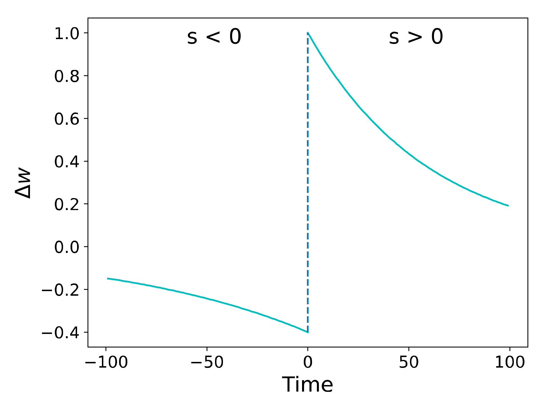
Spike-timing-dependent plasticity (STDP) [17,18] is, probably, the most fundamental form of the unsupervised learning rule observed in biology. It is closely related to Hebb’s postulate: “Neurons that fire together, wire together” [19]. The hypothesis underlying the STDP rule is that the change in the weight of a synapse between two neurons is proportional to the separation between pre- and postsynaptic spike times. If the postsynaptic spike occurs after a presynaptic spike, then the change in the weight of the synapse is positive (i.e., weight is increased), thereby strengthening the causal relationship between the pre- and postsynaptic spikes. On the other hand, if the presynaptic spike occurs after a postsynaptic spike, then the change in the weight of the synapse is negative (i.e., weight is reduced), thereby further weakening the causal relationship between the pre- and postsynaptic spikes. Furthermore, in both cases, the change in the weight is negatively correlated with the difference between the pre- and postsynaptic spike times, i.e., the change in weight is smaller for higher values of the difference between the spike times of the pre- and postsynaptic neurons. The change in weight of a synapse based on STDP is given by
where and represent the coefficients for potentiation and depression, and and represent the time constants for STDP in the respective cases. is the time difference between the spike times of the post- and presynaptic neuron. Figure 1 shows the relationship between the change in weight and for given values of different parameters associated with STDP.
STDP is the basis of many unsupervised learning approaches for SNNs, most of which use the learned representations for classification tasks. STDP is used along with lateral inhibition and an adaptive spiking threshold to learn representations for input spike patterns that are suitable for classification [20]. Based on the representations learnt using STDP, an accuracy of 95% is reported on the MNIST dataset. Several approaches have also used STDP in combination with winner-take-all approaches to learn representations that are suitable for classification [21].
4.2. Supervized Learning
Supervized learning in SNNs focuses on adapting the network parameters to minimize some formulation of error based on a network’s actual output spike pattern and the desired output spike pattern. The value that is represented by the desired output spike pattern depends on the task being handled by the network. For instance, in a classification task, desired output spike patterns encode the class label associated with a given sample, whereas, in regression tasks, it encodes a real value. Depending on the fundamental principles of a learning algorithm, the supervised learning approaches for SNNs can be classified into the following categories: gradient-based learning, bio-inspired learning and other learning algorithms. Below, we look at each of the categories separately.
4.2.1. Gradient-Based Learning
The general idea behind gradient-based approaches is to update weights in the network based on the gradient of an error function. The success of gradient-based algorithms for ANNs has inspired the development of many similar approaches for SNNs. These approaches have focused on the development of better techniques for computing gradients at the time of spike, which cannot be computed analytically because of the discontinuity in the neuronal response [8]. SpikeProp is one of the first gradient-based learning approaches for SNNs that computes a gradient at the time of spike by assuming that the potential of the neuron changes linearly around this time [8]. In [22], authors employed low-pass filtering to smoothen the changes in the membrane potential of the neuron around the time of spike, thereby enabling computation of the gradient. Recently, the concept of surrogate gradients in spiking neural networks has been proposed, which involves replacing each spike in the network by a continuous differentiable function [23]. The effectiveness of surrogate gradients in training deep neural networks have led to their utilization in a large number of recent studies [24,25,26].
4.2.2. Bio-Inspired Learning
Bio-inspired learning algorithms are based on learning strategies which are observed in the brain (such as STDP) or utilize an observation from biology as a foundational idea (such as rank-order coding [27]). Most bio-inspired approaches have focused on shallow two-layered SNNs [28,29] or utilized layer-wise training [30,31] due to a lack of understanding about how learning occurs across hierarchical networks in the brain. Many studies based on shallow SNNs have proposed approaches that combine STDP with a supervisory signal to train SNNs [28,29]. In [29], STDP is combined with the Bienenstock–Cooper–Munro learning rule to modulate the height of the plasticity window associated with STDP. In [28], STDP is used to train a network that utilizes synapses with time-varying weights. Layer-wise training approaches train a deep network layer-by-layer, which alleviates the need for computation of gradients for back propagation. A layer-wise training approach that utilizes a local learning rule was developed to train a three-layer SNN for classification tasks in [32]. Kheradpisheh et al. proposed an STDP-based layer-wise training approach for a deep neural network [30]. The representations inferred in the last layer of the network are used for image classification.
To overcome issues pertaining to longer training times associated with layer-wise training algorithms, some studies have proposed techniques that combine gradient-based approaches with bio-inspired learning rules. In [33], STDP is combined with a gradient-based approach to train deep SNNs. To overcome issues arising because of the discontinuity around spikes, the application of gradient descent is limited to small intervals with zero or one spike. In [34], authors combined STDP with self-regulation to develop a learning algorithm that can use different learning strategies depending on the error in the network’s response for a given spike pattern.
Bio-inspired learning approaches such as STDP and rank-order learning have also been employed for the development of training algorithms for evolving SNNs. Evolving spiking neural networks (eSNN) use rank-order learning based on the first spikes generated by neurons in the network for learning and evolving the network [35]. Dynamic eSNN is an extension of eSNN that uses the first spike for evolving the network but uses all spikes for adapting the weights [36]. Learning in Dynamic eSNN is conducted using the spike-driven synaptic plasticity learning rule, which is a variant of the STDP.
4.2.3. Other Learning Algorithms
This category represents a class of algorithms that are neither reliant on gradients nor utilize learning mechanisms observed in biology for training SNNs. In [32], the authors developed a learning rule that utilizes the normalized contributions of the presynaptic neurons towards the spikes generated by postsynaptic neurons for learning. Chronotron utilizes the Victor and Purpura distance metric for spike patterns to develop a local learning rule for training shallow SNNs [37]. The learning rule in Chronotron utilizes the difference between synaptic current due to actual presynaptic spikes and desired spikes for learning. SPAN convolves the spike patterns generated by input neurons with a continuous function and then utilizes the Widrow–Hoff learning rule to update the synaptic weights in a two-layered SNN [38]. SPAN is an algorithm that trains a spiking neuron to generate a sequence of output spikes at desired future times. It is a supervised learning algorithm where time is not only represented in the input spike sequences but also learned in the spike output sequences generated by the spiking neuron.
4.3. Reinforcement Learning
Reinforcement learning (RL) involves adapting the parameters of an SNN based on external feedback that depends on the predictions generated by the network. RL has not yet received significant attention in the field of SNNs. One of the well-known approaches for RL using SNNs is reward-modulated STDP, which has been utilized in multiple studies [39,40]. Recently, policy gradients have been used to develop a reinforcement learning approach for SNNs [41]. The approach models each spiking neuron as a generalized linear model to overcome issues associated with the computation of gradients in SNNs.
5. Generic Applications of SNN in Computational Intelligence
In principle, SNNs can be used for all the applications that an artificial neural network can be used for. However, the binary nature of spikes renders SNNs more energy efficient and faster with regards to response latency in comparison to ANNs. Furthermore, the temporal nature of spikes renders SNNs more suitable for the processing of spatiotemporal inputs. In this section, we present a brief survey of generic applications of SNNs, followed by a more detailed overview of applications focusing on SNNs realized using neuromorphic chips in Section 6 and the applications of specific brain-inspired SNN architectures in Section 7.
With regards to supervised learning, many studies have reported performance on benchmark datasets such as MNIST and CIFAR-10 for classification tasks [22,26,31]. The most significant applications of SNNs involve directly utilizing the sensor data received from dynamic vision sensors. Dynamic vision sensors are more sensitive to visual changes and have very low power requirements [42]. This is particularly useful for development of energy-efficient, end-to-end processing pipelines with low response latency.
Recently, many of the applications of SNNs have focused on RL, as it is generally easier to frame real-world problems, such as robot control, as an RL task. In [43], an end-to-end SNN-based approach was proposed for a lane-keeping vehicle. The approach directly utilizes the spike-based input received from the neuromorphic vision sensor on a simulated pioneer robot to train it for performing a right-lane-keeping task. The SNN is trained using STDP modulated according to the reward received by the agent for its actions. In [44], the authors developed a multiplicative version of the reward-modulated STDP for training an agent for collision avoidance using reinforcement learning.
6. SNNs on Neuromorphic Chips
Most likely, the most significant advantage of SNNs in comparison to artificial neural networks is their potential to perform energy-efficient computing, due to the way information is represented in SNNs. Here, energy efficiency refers to the power requirements of the hardware used to simulate a SNN. The binary and sparse nature of spikes renders SNNs suitable for edge-based computing, i.e., devices with limited on-board power. However, due to the lack of effective means for porting software implementations of SNNs to hardware, there have been limited efforts in using SNNs for real-world applications. The research in this direction is mainly driven by the capabilities of the neuromorphic chips for realizing SNNs in hardware.
Loihi is a neuromorphic chip developed by Intel using its 14 nm process [45]. The first version of the chip was able to simulate 130,000 neurons and 130 million synapses while consuming 35 to 140 watts of power [45]. The Loihi chip has a form factor of USB, which makes it ideal for applications where it is not feasible to install high-performance computing infrastructure, for instance, unmanned aerial vehicles (UAV). In [46], the low-power computing capabilities of the Loihi chip were exploited to develop a functional PID controller for a UAV with one degree of freedom. In [47], the Loihi chip was used to develop an optic-flow based approach for autonomous landing of UAVs. Recently, the chip was used by researchers at the University of Zurich to develop a high-speed controller for UAV [48]. A more rigorous survey of Loihi applications was provided in [49].
TrueNorth is a neuromorphic chip developed by IBM that operates using 70 milliwatts of power [50], which is much closer to the energy requirements of the brain. The TrueNorth chip can simulate up to 1 million programmable neurons and 256 million programmable synapses. However, a single neuron on the TrueNorth chip can have at most 256 synapses. The extremely low energy footprint of the TrueNorth chip has made it useful for applications where charging cycles can be very long, for instance, in wearables devices. In [51], a TrueNorth chip was used for decoding the electroencephalogram (EEG) and local field potential (LFP) signals observed in the brain. In [52], an image segmentation approach, realized on TrueNorth, was used for identifying the spinal anatomy in images obtained using medical resonance imaging. In [53], the TrueNorth chip was used to develop an end-to-end neuromorphic framework for object detection and tracking in a surveillance application.
Besides Loihi and TrueNorth, there are several other neuromorphic hardwares which have been developed with the aim of improving the performance of existing alternatives. SpiNNaker [54], BrainScaleS [55] and Neurogrid [56] were developed with a focus on efficient and faster simulations for neuroscientific studies. FlexLearn [57] provides a general framework to support brain simulations with on-chip learning based on a multitude of plasticity mechanisms observed in the brain. SpinalFlow [58] developed an efficient method to compute the potential of a spiking neuron to improve the throughput of existing neuromorphic hardwares. NEBULA [59] employs a magnetic tunnel junction that can simulate both synapses as well as neurons with ultra-low voltage requirements. These advances have resulted in the development of efficient hardware solutions for simulated SNNs. The adoption of these solutions on a wider scale could be further accelerated through collaborative efforts between hardware groups and researchers focusing on developing learning approaches for SNNs. Neuromorphic chips have also been utilized for purposes that do not require SNNs but can benefit from the energy-efficient information propagation mechanism of spiking neurons. Such applications are beyond the scope of this article, but a detailed review on this topic has been presented in [60].
7. Future Trends: Brain-Inspired SNN Architectures
One aspect of brain-inspired SNN (BI-SNN) architectures is the use of a brain template to structure a 3D SNN structure that is trained on spike sequence data [15]. Such a brain-template could be Talairach [61], MNI, MRI [62] or other brain structural information.
7.1. The NeuCube Architecture
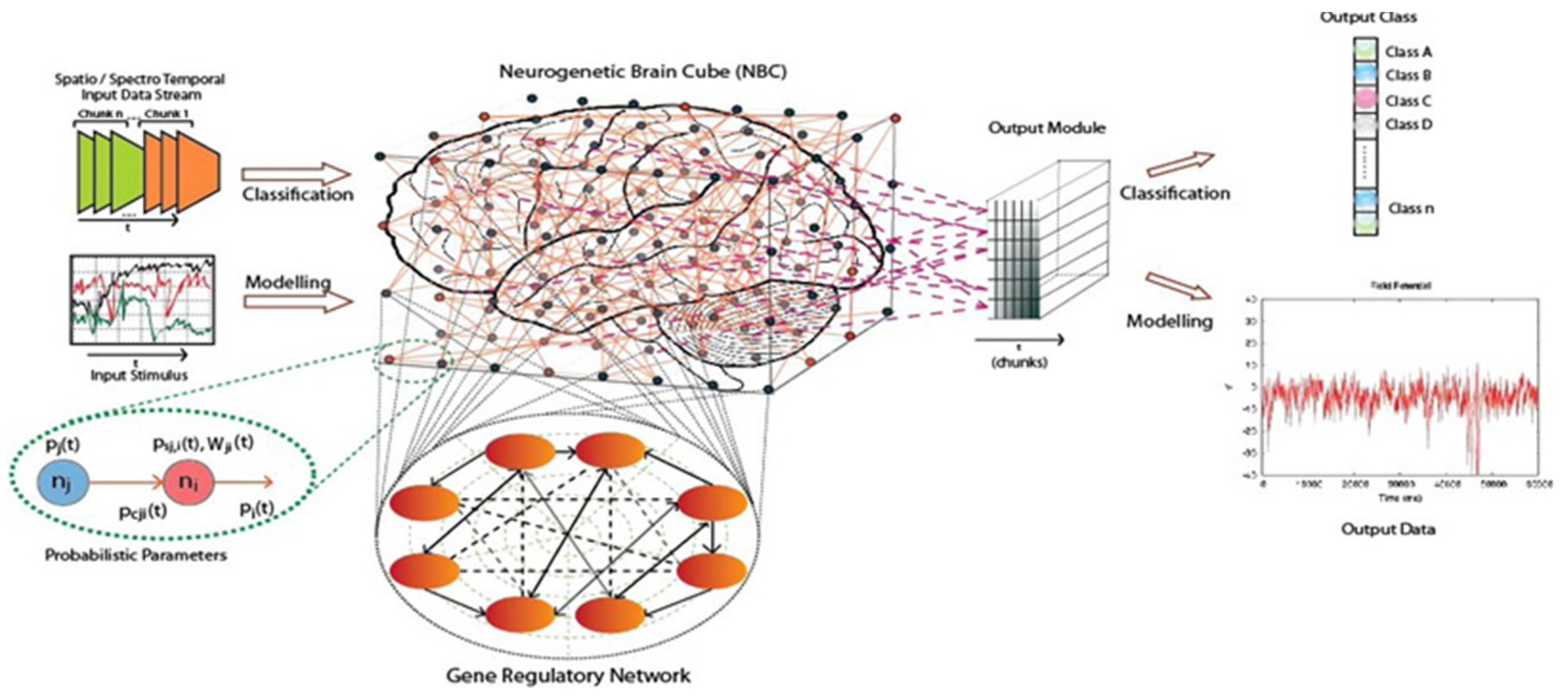
NeuCube is a BI-SNN, which was originally developed for modelling spatio-temporal data obtained from the brain but has since been used for a variety of applications, such as climate data modelling and stroke prediction. The architecture of NeuCube is shown in Figure 2. The main parts (modules) of NeuCube are:
- -
- Input information encoding module;
- -
- 3D SNN reservoir/cube module (SNNc), or also neurogenetic brain cube (NBC), for unsupervised learning;
- -
- Output classification/regression module for supervised learning;
- -
- Gene regulatory network module (optional).
NeuCube utilizes three types of mutually interacting memories, which are:
- -
- Short-term memory, represented as changes of the membrane potential level and temporary changes of synaptic efficacy;
- -
- Long-term memory, represented as a stable establishment of synaptic efficacy—LTP and LTD;
- -
- Genetic memory, represented as a genetic code.
Short term memory in NeuCube is represented via similar activation patterns, termed as ‘polychronous waves’ in the SNNs with recurrent connections. The weights of the synaptic connections can be updated using LTP or LTD. NeuCube can be used for studying/learning long spatio-temporal patterns and for building associative memories. At the end of training, NeuCube retains the connections which represent long-term memory in NeuCube. Current applications of NeuCube include:
- -
- Predicting brain re-wiring through mindfulness [63];
- -
- Modelling neuroimaging data such as EEG and fMRI [62];
- -
- Personalized brain data modelling [64];
- -
- Emotion recognition [65];
- -
- Speech, sound and music recognition [66];
- -
- Moving object recognition [67];
- -
- Prediction of events from temporal climate data (stroke) [64];
- -
- Brain–computer interfaces (BCI) [68].
7.2. Integration of Multimodal Data in a BI-SNN Architectures
As the brain integrates multiple input stimuli into one learning system, a BI-SNN can also be used for such integration. Examples are:
- -
- Integrating time, space and orientation data, such as fMRI and DTI [66,69]: An extension of the STDP learning rule was proposed in [69], called oiSTDP, where if two or more postsynaptic neurons spike after a pre-synaptic neuron, the closer a postsynaptic neuron is to the orientation vector, the higher the increase is in the connection weight of that postsynaptic neuron. The proposed rules are utilized for integrating MRI and DTI data to create a personalized model for predicting the response of schizophrenic patient to clozapine. Based on the proposed approach, it has been shown that higher prediction accuracy is achieved using the integrated data;
- -
- -
- Integrating genetic data into a neurogenetic SNN architecture [70]: In [70], a gene interaction network model was suggested as part of a spiking neuron model based on the neuroreceptors AMPAR and NMDAR. For a given problem, such as modelling AD, genes can be connected to these neuroreceptors in a gene regulatory network, thereby influencing the performance of the SNN as a whole.
8. Conclusions
In this article, we have presented an overview of the recent technical advances pertaining to SNNs and their usage in real-world applications. Based on this, we have also identified interesting future trends and directions of research. The natural capabilities of spiking neurons to represent temporal information renders them suitable for processing spatio-temporal data arising in various domains such as brain and cognitive data analytics, brain-computer interfaces, knowledge transfer between humans and machines, brain-like robotics, incremental and transfer learning of multisensory streaming data. Further evaluation and appreciation of the advantages of SNNs are expected in terms of energy-efficiency, response latency and explainability [68]. Further development in SNN is expected in many directions, including new neuromorphic chip design [71,72], on-line and real-time applications, predictive modelling of brain diseases and the integration of new knowledge from bioinformatics and neuroinformatics. Dedicated research in these directions would contribute towards the identification of other suitable areas where neuromorphic computing could offer substantial advantages over traditional ANNs, thereby accelerating research on SNNs.
Author Contributions
Conceptualization, S.D. and N.K.; writing—original draft preparation, S.D.; writing—review and editing, S.D. and N.K. All authors have read and agreed to the published version of the manuscript.
Funding
This research received no external funding.
Institutional Review Board Statement
Not applicable.
Informed Consent Statement
Not applicable.
Data Availability Statement
The data supporting the reported results in the present study will be available on request from the corresponding author or the first author.
Conflicts of Interest
The authors declare no conflict of interest.
References
- Du, Z.; Rubin, D.D.B.-D.; Chen, Y.; He, L.; Chen, T.; Zhang, L.; Wu, C.; Temam, O. Neuromorphic accelerators. In Proceedings of the 48th International Symposium on Microarchitecture, Waikiki, HI, USA, 5–9 December 2015; pp. 494–507. [Google Scholar]
- Deng, L.; Wu, Y.; Hu, X.; Liang, L.; Ding, Y.; Li, G.; Zhao, G.; Li, P.; Xie, Y. Rethinking the performance comparison between SNNS and ANNS. Neural Netw. 2020, 121, 294–307. [Google Scholar] [CrossRef] [PubMed]
- Lee, H.; Kim, C.; Lee, S.; Baek, E.; Kim, J. An accurate and fair evaluation methodology for SNN-based inferencing with full-stack hardware design space explorations. Neurocomputing 2021, 455, 125–138. [Google Scholar] [CrossRef]
- Hodgkin, A.L.; Huxley, A.F. A quantitative description of membrane current and its application to conduction and excitation in nerve. J. Physiol. 1952, 117, 500–544. [Google Scholar] [CrossRef] [PubMed]
- Abbott, L.F. Lapicque’s introduction of the integrate-and-fire model neuron (1907). Brain Res. Bull. 1999, 50, 303–304. [Google Scholar] [CrossRef]
- Izhikevich, E. Simple model of spiking neurons. IEEE Trans. Neural Networks 2003, 14, 1569–1572. [Google Scholar] [CrossRef] [Green Version]
- Gerstner, W.; Kistler, W.M. Spiking Neuron Models: Single Neurons, Populations, Plasticity; Cambridge University Press: Cambridge, UK, 2002. [Google Scholar]
- Bohte, S.M.; Kok, J.N.; La Poutré, H. Error-backpropagation in temporally encoded networks of spiking neurons. Neurocomputing 2002, 48, 17–37. [Google Scholar] [CrossRef] [Green Version]
- She, X.; Dash, S.; Kim, D.; Mukhopadhyay, S. A Heterogeneous Spiking Neural Network for Unsupervised Learning of Spatiotemporal Patterns. Front. Neurosci. 2021, 14, 1406. [Google Scholar] [CrossRef]
- Srinivasa, N.; Cho, Y. Self-Organizing Spiking Neural Model for Learning Fault-Tolerant Spatio-Motor Transformations. IEEE Trans. Neural Networks Learn. Syst. 2012, 23, 1526–1538. [Google Scholar] [CrossRef]
- Kandel, E.R.; Mack, S.; Jessell, T.M.; Schwartz, J.H.; Siegelbaum, S.A.; Hudspeth, A.J. Principles of Neural Science, 5th ed.; McGraw Hill Professional: New York, NY, USA, 2013. [Google Scholar]
- Dora, S.; Suresh, S.; Sundararajan, N. A sequential learning algorithm for a Minimal Spiking Neural Network (MSNN) classifier. In Proceedings of the 2014 International Joint Conference on Neural Networks (IJCNN), Beijing, China, 6–11 July 2014; pp. 2415–2421. [Google Scholar]
- Wang, J.; Belatreche, A.; Maguire, L.; McGinnity, T.M. An online supervised learning method for spiking neural networks with adaptive structure. Neurocomputing 2014, 144, 526–536. [Google Scholar] [CrossRef]
- Dora, S.; Suresh, S.; Sundararajan, N. Online Meta-neuron based Learning Algorithm for a spiking neural classifier. Inf. Sci. 2017, 414, 19–32. [Google Scholar] [CrossRef]
- Kasabov, N.K. NeuCube: A spiking neural network architecture for mapping, learning and understanding of spatio-temporal brain data. Neural Netw. 2014, 52, 62–76. [Google Scholar] [CrossRef]
- Hazan, H.; Saunders, D.J.; Khan, H.; Patel, D.; Sanghavi, D.T.; Siegelmann, H.T.; Kozma, R. BindsNET: A Machine Learning-Oriented Spiking Neural Networks Library in Python. Front. Aging Neurosci. 2018, 12, 89. [Google Scholar] [CrossRef]
- Markram, H.; Lübke, J.; Frotscher, M.; Sakmann, B. Regulation of Synaptic Efficacy by Coincidence of Postsynaptic APs and EPSPs. Sci. 1997, 275, 213–215. [Google Scholar] [CrossRef] [Green Version]
- Bi, G.-Q.; Poo, M.-M. Synaptic Modifications in Cultured Hippocampal Neurons: Dependence on Spike Timing, Synaptic Strength, and Postsynaptic Cell Type. J. Neurosci. 1998, 18, 10464–10472. [Google Scholar] [CrossRef]
- Hebb, D.O. The Organization of Behavior: A Neuropsychological Theory; Wiley: New York, NY, USA, 1949. [Google Scholar]
- Diehl, P.U.; Cook, M. Unsupervised learning of digit recognition using spike-timing-dependent plasticity. Front. Comput. Neurosci. 2015, 9, 99. [Google Scholar] [CrossRef] [Green Version]
- Ferré, P.; Mamalet, F.; Thorpe, S. Unsupervised Feature Learning With Winner-Takes-All Based STDP. Front. Comput. Neurosci. 2018, 12, 24. [Google Scholar] [CrossRef] [Green Version]
- Lee, J.H.; Delbruck, T.; Pfeiffer, M. Training Deep Spiking Neural Networks Using Backpropagation. Front. Neurosci. 2016, 10, 508. [Google Scholar] [CrossRef] [Green Version]
- Neftci, E.O.; Mostafa, H.; Zenke, F. Surrogate Gradient Learning in Spiking Neural Networks: Bringing the Power of Gradient-Based Optimization to Spiking Neural Networks. IEEE Signal Process. Mag. 2019, 36, 51–63. [Google Scholar] [CrossRef]
- Zenke, F.; Vogels, T.P. The Remarkable Robustness of Surrogate Gradient Learning for Instilling Complex Function in Spiking Neural Networks. Neural Comput. 2021, 33, 899–925. [Google Scholar] [CrossRef]
- Panda, P.; Aketi, S.A.; Roy, K. Toward Scalable, Efficient, and Accurate Deep Spiking Neural Networks With Backward Residual Connections, Stochastic Softmax, and Hybridization. Front. Neurosci. 2020, 14, 653. [Google Scholar] [CrossRef]
- Shrestha, S.B.; Orchard, G. SLAYER: Spike Layer Error Reassignment in Time. Available online: http://papers.nips.cc/paper/7415-slayer-spike-layer-error-reassignment-in-time.pdf (accessed on 15 October 2019).
- Thorpe, S.; Gautrais, J. Rank Order Coding. In Computational Neuroscience; Plenum press: New York, NY, USA, 1998. [Google Scholar]
- Jeyasothy, A.; Sundaram, S.; Sundararajan, N. SEFRON: A New Spiking Neuron Model With Time-Varying Synaptic Efficacy Function for Pattern Classification. IEEE Trans. Neural Networks Learn. Syst. 2018, 30, 1231–1240. [Google Scholar] [CrossRef] [PubMed]
- Wade, J.J.; McDaid, L.J.; Santos, J.A.; Sayers, H.M. SWAT: A Spiking Neural Network Training Algorithm for Classification Problems. IEEE Trans. Neural Netw. 2010, 21, 1817–1830. [Google Scholar] [CrossRef] [Green Version]
- Kheradpisheh, S.R.; Ganjtabesh, M.; Thorpe, S.J.; Masquelier, T. STDP-based spiking deep convolutional neural networks for object recognition. Neural Netw. 2018, 99, 56–67. [Google Scholar] [CrossRef] [Green Version]
- Lee, C.; Srinivasan, G.; Panda, P.; Roy, K. Deep Spiking Convolutional Neural Network Trained With Unsupervised Spike-Timing-Dependent Plasticity. IEEE Trans. Cogn. Dev. Syst. 2019, 11, 384–394. [Google Scholar] [CrossRef]
- Dora, S.; Sundaram, S.; Sundararajan, N. An Interclass Margin Maximization Learning Algorithm for Evolving Spiking Neural Network. IEEE Trans. Cybern. 2018, 49, 989–999. [Google Scholar] [CrossRef]
- Tavanaei, A.; Maida, A.S. Bio-Inspired Spiking Convolutional Neural Network using Layer-wise Sparse Coding and STDP Learning. Available online: http://arxiv.org/abs/1611.03000 (accessed on 5 January 2020).
- Machingal, P.; Thousif, M.; Dora, S.; Sundaram, S. Self-regulated Learning Algorithm for Distributed Coding Based Spiking Neural Classifier. In Proceedings of the 2020 International Joint Conference on Neural Networks (IJCNN), Glasgow, UK, 19–24 July 2020; pp. 1–7. [Google Scholar]
- Wysoski, S.G.; Benuskova, L.; Kasabov, N. Fast and adaptive network of spiking neurons for multi-view visual pattern recognition. Neurocomputing 2008, 71, 2563–2575. [Google Scholar] [CrossRef]
- Kasabov, N.; Dhoble, K.; Nuntalid, N.; Indiveri, G. Dynamic evolving spiking neural networks for on-line spatio- and spectro-temporal pattern recognition. Neural Netw. 2013, 41, 188–201. [Google Scholar] [CrossRef] [PubMed] [Green Version]
- Florian, R.V. The Chronotron: A Neuron That Learns to Fire Temporally Precise Spike Patterns. PLOS ONE 2012, 7, e40233. [Google Scholar] [CrossRef] [PubMed] [Green Version]
- Mohemmed, A.; Schliebs, S.; Matsuda, S.; Kasabov, N. Span: Spike Pattern Association Neuron for Learning Spatio-Temporal Spike Patterns. Int. J. Neural Syst. 2012, 22, 1250012. [Google Scholar] [CrossRef] [PubMed]
- Florian, R.V. Reinforcement Learning Through Modulation of Spike-Timing-Dependent Synaptic Plasticity. Neural Comput. 2007, 19, 1468–1502. [Google Scholar] [CrossRef] [PubMed] [Green Version]
- Zheng, N.; Mazumder, P. Hardware-Friendly Actor-Critic Reinforcement Learning Through Modulation of Spike-Timing-Dependent Plasticity. IEEE Trans. Comput. 2016, 66, 299–311. [Google Scholar] [CrossRef]
- Rosenfeld, B.; Simeone, O.; Rajendran, B. Learning First-to-Spike Policies for Neuromorphic Control Using Policy Gradients. In Proceedings of the 2019 IEEE 20th International Workshop on Signal Processing Advances in Wireless Communications (SPAWC), Cannes, France, 2–5 July 2019; pp. 1–5. [Google Scholar]
- Falanga, D.; Kleber, K.; Scaramuzza, D. Dynamic obstacle avoidance for quadrotors with event cameras. Sci. Robot. 2020, 5, 9712. [Google Scholar] [CrossRef]
- Bing, Z.; Meschede, C.; Huang, K.; Chen, G.; Rohrbein, F.; Akl, M.; Knoll, A. End to End Learning of Spiking Neural Network Based on R-STDP for a Lane Keeping Vehicle. In Proceedings of the 2018 IEEE International Conference on Robotics and Automation (ICRA), Brisbane, QLD, Australia, 21–25 May 2018; pp. 1–8. [Google Scholar]
- Shim, M.S.; Li, P. Biologically inspired reinforcement learning for mobile robot collision avoidance. In Proceedings of the 2017 International Joint Conference on Neural Networks (IJCNN), Anchorage, AK, USA, 14–19 May 2017; pp. 3098–3105. [Google Scholar]
- Nast, C.; The future of AI is neuromorphic. Meet the Scientists Building Digital “Brains” for Your Phone. Available online: https://www.wired.co.uk/article/ai-neuromorphic-chips-brains (accessed on 12 September 2021).
- Stagsted, R.; Vitale, A.; Binz, J.; Renner, A.; Larsen, L.B.; Sandamirskaya, Y. Towards neuromorphic control: A spiking neural network based PID controller for UAV. In Proceedings of the Robotics: Science and Systems XVI, Corvalis, OR, USA, 12–16 July 2020. [Google Scholar]
- Dupeyroux, J.; Hagenaars, J.J.; Paredes-Valles, F.; de Croon, G.C.H.E. Neuromorphic control for optic-flow-based landing of MAVs using the Loihi processor. In Proceedings of the 2021 IEEE International Conference on Robotics and Automation (ICRA), Xi’an, China, 30 May–5 June 2021; pp. 96–102. [Google Scholar]
- Vitale, A.; Renner, A.; Nauer, C.; Scaramuzza, D.; Sandamirskaya, Y. Event-driven Vision and Control for UAVs on a Neuromorphic Chip. In Proceedings of the 2021 IEEE International Conference on Robotics and Automation (ICRA), Xi’an, China, 30 May–5 June 2021; pp. 103–109. [Google Scholar]
- Davies, M.; Wild, A.; Orchard, G.; Sandamirskaya, Y.; Guerra, G.A.F.; Joshi, P.; Plank, P.; Risbud, S.R. Advancing Neuromorphic Computing With Loihi: A Survey of Results and Outlook. Proc. IEEE 2021, 109, 911–934. [Google Scholar] [CrossRef]
- Merolla, P.A.; Arthur, J.V.; Alvarez-Icaza, R.; Cassidy, A.S.; Sawada, J.; Akopyan, F.; Jackson, B.L.; Imam, N.; Guo, C.; Nakamura, Y.; et al. A million spiking-neuron integrated circuit with a scalable communication network and interface. Science 2014, 345, 668–673. [Google Scholar] [CrossRef]
- Nurse, E.; Mashford, B.S.; Yepes, A.J.; Kiral-Kornek, I.; Harrer, S.; Freestone, D.R. Decoding EEG and LFP signals using deep learning. In Proceedings of the ACM International Conference on Computing Frontiers, Como, Italy, 16–19 May 2016; pp. 259–266. [Google Scholar]
- Moran, S.; Gaonkar, B.; Macyszyn, L.; Whitehead, W.; Wolk, A.; Iyer, S.S. Deep learning for medical image segmentation – using the IBM TrueNorth neurosynaptic system. In Proceedings of the Medical Imaging 2018: Imaging Informatics for Healthcare, Research, and Applications, Houston, TX, USA, 10–15 February 2018. [Google Scholar]
- Ussa, A.; Vedova, L.D.; Padala, V.R.; Singla, D.; Acharya, J.; Lei, C.Z.; Orchard, G.; Basu, A.; Ramesh, B. A Low-Power End-to-End Hybrid Neuromorphic Framework for Surveillance Applications. Available online: http://arxiv.org/abs/1910.09806 (accessed on 12 September 2021).
- Jin, X.; Furber, S.B.; Woods, J.V. Efficient modelling of spiking neural networks on a scalable chip multiprocessor. In Proceedings of the 2008 IEEE International Joint Conference on Neural Networks (IEEE World Congress on Computational Intelligence), Hong Kong, China, 1–8 June 2008; pp. 2812–2819. [Google Scholar]
- Schemmel, J.; Briiderle, D.; Griibl, A.; Hock, M.; Meier, K.; Millner, S. A wafer-scale neuromorphic hardware system for large-scale neural modeling. In Proceedings of the 2010 IEEE International Symposium on Circuits and Systems, Paris, France, 30 May–2 June 2010; pp. 1947–1950. [Google Scholar]
- Benjamin, B.V.; Gao, P.; McQuinn, E.; Choudhary, S.; Chandrasekaran, A.R.; Bussat, J.-M.; Alvarez-Icaza, R.; Arthur, J.V.; Merolla, P.A.; Boahen, K. Neurogrid: A Mixed-Analog-Digital Multichip System for Large-Scale Neural Simulations. Proc. IEEE 2014, 102, 699–716. [Google Scholar] [CrossRef]
- Baek, E.; Lee, H.; Kim, Y.; Kim, J. FlexLearn: Fast and Highly Efficient Brain Simulations Using Flexible On-Chip Learning. In Proceedings of the 52nd Annual IEEE/ACM International Symposium on Microarchitecture, Columbus, OH, USA, 12–16 October 2019; pp. 304–318. [Google Scholar]
- Narayanan, S.; Taht, K.; Balasubramonian, R.; Giacomin, E.; Gaillardon, P.-E. SpinalFlow: An Architecture and Dataflow Tailored for Spiking Neural Networks. In Proceedings of the 2020 ACM/IEEE 47th Annual International Symposium on Computer Architecture (ISCA), Valencia, Spain, 30 May–3 June 2020; pp. 349–362. [Google Scholar]
- Singh, S.; Sarma, A.; Jao, N.; Pattnaik, A.; Lu, S.; Yang, K.; Sengupta, A.; Narayanan, V.; Das, C.R. NEBULA: A Neuromorphic Spin-Based Ultra-Low Power Architecture for SNNs and ANNs. In Proceedings of the 2020 ACM/IEEE 47th Annual International Symposium on Computer Architecture (ISCA), Valencia, Spain, 30 May–3 June 2020; pp. 363–376. [Google Scholar]
- Aimone, J.B.; Hamilton, K.E.; Mniszewski, S.; Reeder, L.; Schuman, C.D.; Severa, W.M. Non-Neural Network Applications for Spiking Neuromorphic Hardware. Available online: https://sc18.supercomputing.org/proceedings/workshops/workshop_files/ws_pmes105s1-file1.pdf (accessed on 12 September 2021).
- Talairach, J.; Tournoux, P. Co-planar Stereotaxic Atlas of the Human Brain; Thieme Medical Publishers: New York, NY, USA, 1998. [Google Scholar]
- Saeedinia, S.A.; Jahed-Motlagh, M.R.; Tafakhori, A.; Kasabov, N. Design of MRI structured spiking neural networks and learning algorithms for personalized modelling, analysis, and prediction of EEG signals. Sci. Rep. 2021, 11, 1–14. [Google Scholar] [CrossRef]
- Doborjeh, Z.; Doborjeh, M.; Taylor, T.; Kasabov, N.; Wang, G.Y.; Siegert, R.; Sumich, A. Spiking Neural Network Modelling Approach Reveals How Mindfulness Training Rewires the Brain. Sci. Rep. 2019, 9, 1–15. [Google Scholar] [CrossRef]
- Kasabov, N.; Feigin, V.L.; Hou, Z.-G.; Chen, Y.; Liang, L.; Krishnamurthi, R.; Othman, M.; Parmar, P. Evolving spiking neural networks for personalised modelling, classification and prediction of spatio-temporal patterns with a case study on stroke. Neurocomputing 2014, 134, 269–279. [Google Scholar] [CrossRef] [Green Version]
- Tan, C.; Šarlija, M.; Kasabov, N. NeuroSense: Short-term emotion recognition and understanding based on spiking neural network modelling of spatio-temporal EEG patterns. Neurocomputing 2021, 434, 137–148. [Google Scholar] [CrossRef]
- Kasabov, N.K. Time-Space, Spiking Neural Networks and Brain-Inspired Artificial Intelligence; Springer: Dordrecht, Netherlands, 2019. [Google Scholar]
- Paulun, L.; Wendt, A.; Kasabov, N. A Retinotopic Spiking Neural Network System for Accurate Recognition of Moving Objects Using NeuCube and Dynamic Vision Sensors. Front. Comput. Neurosci. 2018, 12, 42. [Google Scholar] [CrossRef]
- Kumarasinghe, K.; Kasabov, N.; Taylor, D. Brain-inspired spiking neural networks for decoding and understanding muscle activity and kinematics from electroencephalography signals during hand movements. Sci. Rep. 2021, 11, 1–15. [Google Scholar] [CrossRef] [PubMed]
- Sengupta, N.; McNabb, C.; Kasabov, N.; Russell, B.R. Integrating Space, Time, and Orientation in Spiking Neural Networks: A Case Study on Multimodal Brain Data Modeling. IEEE Trans. Neural Networks Learn. Syst. 2018, 29, 5249–5263. [Google Scholar] [CrossRef] [PubMed]
- Benuskova, L.; Kasabov, N. Computational Neurogenetic Modeling; Springer Science and Business Media: New York, NY, USA, 2007. [Google Scholar]
- Furber, S. To build a brain. IEEE Spectr. 2012, 49, 44–49. [Google Scholar] [CrossRef]
- Indiveri, G.; Linares-Barranco, B.; Hamilton, T.J.; van Schaik, A.; Etienne-Cummings, R.; Delbruck, T.; Liu, S.-C.; Dudek, P.; Häfliger, P.; Renaud, S.; et al. Neuromorphic Silicon Neuron Circuits. Front. Behav. Neurosci. 2011, 5, 73. [Google Scholar] [CrossRef] [Green Version]
Figure 1.
Relationship between the change in weight of a synapse and the difference between spike times of the pre- and postsynaptic neurons. where and represent the spike times for the pre- and postsynaptic neurons, respectively. Figure was generated using the following values: , , and .
Figure 1.
Relationship between the change in weight of a synapse and the difference between spike times of the pre- and postsynaptic neurons. where and represent the spike times for the pre- and postsynaptic neurons, respectively. Figure was generated using the following values: , , and .

Figure 2.
A schematic diagram of the NeuCube architecture (adopted from [15]).
Figure 2.
A schematic diagram of the NeuCube architecture (adopted from [15]).

Publisher’s Note: MDPI stays neutral with regard to jurisdictional claims in published maps and institutional affiliations. |
© 2021 by the authors. Licensee MDPI, Basel, Switzerland. This article is an open access article distributed under the terms and conditions of the Creative Commons Attribution (CC BY) license (https://creativecommons.org/licenses/by/4.0/).
Share and Cite
MDPI and ACS Style
Dora, S.; Kasabov, N. Spiking Neural Networks for Computational Intelligence: An Overview. Big Data Cogn. Comput. 2021, 5, 67. https://doi.org/10.3390/bdcc5040067
AMA Style
Dora S, Kasabov N. Spiking Neural Networks for Computational Intelligence: An Overview. Big Data and Cognitive Computing. 2021; 5(4):67. https://doi.org/10.3390/bdcc5040067
Chicago/Turabian StyleDora, Shirin, and Nikola Kasabov. 2021. "Spiking Neural Networks for Computational Intelligence: An Overview" Big Data and Cognitive Computing 5, no. 4: 67. https://doi.org/10.3390/bdcc5040067