


1. Introduction
A shock wave–turbulent boundary layer interaction (STBLI) is a fundamental problem of fluid mechanics, which is also of practical importance in the aerodynamics and propulsion of high-speed flight vehicles (Clemens & Narayanaswamy Reference Clemens and Narayanaswamy2014). A remarkable feature of supersonic STBLIs is a low-frequency, large-scale motion of the flow structure, the source of which is still an open issue.
In addition to the well-known low-frequency back-and-forth motion of the separation shock, the separation bubble exhibits large-scale three-dimensionality. Settles, Fitzpatrick & Bogdonoff (Reference Settles, Fitzpatrick and Bogdonoff1979) conducted a series of compression corner experiments with different ramp angles at a Mach number of M ∞ = 2.85 and a high Reynolds number of Reδ = 1.7 × 10⁶, where δ is the incoming boundary-layer thickness. For the strongest interactions, both the separation and reattachment lines exhibited a zigzag pattern indicated by surface oil flow visualization. A similar flow pattern near reattachment over a 25° compression corner was found by Zheltovodov et al. (Reference Zheltovodov, Trofimov, Schülein and Yakovlev1990) at M ∞ = 2.88 and Reδ = 1.3 × 10⁵. Experiments of impinging shock interactions at M ∞ = 2.3 and Reδ = 5.8 × 10⁴ revealed a three-dimensional (3-D) separation featuring counterrotating streamwise vortices (Dussauge, Dupont & Debiève Reference Dussauge, Dupont and Debiève2006). Zhuang et al. (Reference Zhuang, Tan, Liu, Zhang and Ling2017) observed large-scale streamwise streaks immediately behind the separation shock in a Mach 3 compression corner flow at Reδ = 8.4 × 10⁴ using a Rayleigh scattering technique.
Numerically, streamwise vortices were identified by large-eddy simulations (LES) (Loginov, Adams & Zheltovodov Reference Loginov, Adams and Zheltovodov2006; Grilli et al. Reference Grilli, Schmid, Hickel and Adams2012) under the experimental conditions of Zheltovodov et al. (Reference Zheltovodov, Trofimov, Schülein and Yakovlev1990). Direct numerical simulation of a 24° compression corner interaction at M ∞ = 2.9 and Reδ = 4.4 × 10⁴ showed that the low-frequency shock motion was accompanied by a breathing motion of the separation bubble (Priebe & Martin Reference Priebe and Martin2012). The size of the separation region changed dramatically during the so-called bubble-collapse event. The direct numerical simulation data were further analysed using dynamic mode decomposition by Priebe et al. (Reference Priebe, Tu, Rowley and Martin2016). Unsteady counterrotating streamwise vortices that wander in the spanwise direction were identified. Similar phenomena were found by Pasquariello, Hickel & Adams (Reference Pasquariello, Hickel and Adams2017) using LES in a Mach 3 impinging shock interaction with a strongly separated flow at Reδ = 2 × 10⁵. However, the bubble-collapse event was absent, which was attributed to the much larger separation bubble.
To explain the source of the low-frequency, large-scale unsteadiness, various physical models have been proposed in the literature and can be categorized into two types: upstream and downstream mechanisms (Souverein et al. Reference Souverein, Dupont, Debiève, Dussauge, Van Oudheusden and Scarano2010; Clemens & Narayanaswamy Reference Clemens and Narayanaswamy2014). Ganapathisubramani, Clemens & Dolling (Reference Ganapathisubramani, Clemens and Dolling2007) suggested that the low-frequency unsteadiness was driven by large-scale structures in the incoming boundary layer. Pirozzoli & Grasso (Reference Pirozzoli and Grasso2006) proposed an acoustic feedback model similar to the Rossiter model of cavity resonance (Rossiter Reference Rossiter1964). Piponniau et al. (Reference Piponniau, Dussauge, Debiève and Dupont2009) assumed that shear-layer entrainment resulted in a deficit in the mass of the separation bubble, which was recharged later through the flapping of the shear layer near reattachment. They suggested that such a mass recovery process may be responsible for the low-frequency unsteadiness. More recently, the approach of global stability analysis (GSA) was applied to time- and spanwise-averaged LES data of impinging shock interactions (Touber & Sandham Reference Touber and Sandham2009; Nichols et al. Reference Nichols, Larsson, Bernardini and Pirozzoli2017). A two-dimensional (2-D), zero-frequency, globally unstable mode was captured, which takes the form of bubble expansion/contraction and shock motion. However, the 2-D mean flow obtained from the LES is not an exact solution of any governing equations that can be explicitly expressed, which may result in the unusual zero-frequency unstable mode. Furthermore, only purely 2-D perturbations were considered.
Nonetheless, interpretating the low-frequency unsteadiness as a linear behaviour of large-scale coherent structures from a global stability point of view is very attractive. According to Huerre & Monkewitz (Reference Huerre and Monkewitz1990), a flow is called an oscillator if globally unstable and a noise amplifier if globally stable. An oscillator supports self-excited perturbations and may bifurcate into three-dimensionality and/or unsteadiness. In fact, GSA based on the Reynolds-averaged Navier‒Stokes (RANS) equations has successfully predicted the onset of transonic shock buffet over 2-D airfoils and 3-D wings (Crouch, Garbaruk & Magidov Reference Crouch, Garbaruk and Magidov2007; Crouch et al. Reference Crouch, Garbaruk, Magidov and Travin2009; He & Timme Reference He and Timme2021). In contrast, a noise amplifier feeds on continuous input of external disturbances. Resolvent analysis is usually used to study the dynamics of noise amplifiers, which has also been applied to turbulent flows (Hwang & Cossu Reference Hwang and Cossu2010; McKeon & Sharma Reference Mckeon and Sharma2010). Particularly, the importance of choosing an appropriate eddy viscosity model was highlighted by Pickering et al. (Reference Pickering, Rigas, Schmidt, Sipp and Colonius2021).
In this study, we examine the intrinsic and extrinsic dynamics of STBLIs to reveal the nature of the low-frequency unsteadiness using GSA and resolvent analysis under a unified framework, in which low-frequency, large-scale motions are considered as coherent structures and turbulent fluctuations are closed by turbulence modelling.
2. Geometric configuration and flow conditions
The considered geometry is a compression corner with a ramp angle of α = 25° (see figure 1). A Cartesian coordinate system is constructed with the origin at the corner, the x direction along the flat plate, the y direction perpendicular to the flat plate and the z direction satisfying the right-hand rule. The flow conditions are taken from the experiments of Zheltovodov et al. (Reference Zheltovodov, Trofimov, Schülein and Yakovlev1990). The lowRe case has M ∞ = 2.95 and Reδ = 63 560 with δ = 2.27 mm measured 15.4δ upstream of the corner. The free-stream density is 0.314 kg m−3, and the free-stream temperature is 108 K. The highRe case has M ∞ = 2.88 and Reδ = 132 840 with δ = 4.1 mm measured 8.04δ upstream of the corner. The free-stream density is 0.368 kg m−3, and the free-stream temperature is 114.8 K. The length of the flat plate is determined by matching the experimental boundary-layer thickness for the highRe and lowRe cases, respectively.

Figure 1. Schematic of the geometric configuration and computational domain.
3. Computational details
3.1. Governing equations
The flow is governed by the 3-D compressible RANS equations as
 \begin{equation}\frac{{\partial {\boldsymbol{U}}}}{{\partial t}} = \mathcal{N}({\boldsymbol{U}}),\end{equation}
where U is the vector of conservative variables and  $\mathrm{\mathcal{N}}$ is the nonlinear RANS operator.
Air is modelled as a calorically perfect gas with a specific heat ratio of 1.4 and a Prandtl number of 0.72. Sutherland's law is used to calculate the molecular viscosity. The Reynolds stresses are modelled using the Boussinesq assumption. The eddy viscosity is obtained using the Spalart–Allmaras (S–A) turbulence model (Spalart & Allmaras Reference Spalart and Allmaras1992) with the modification of Edwards & Chandra (Reference Edwards and Chandra1996). The reason why the S–A model is chosen is twofold. First, the length of the separation region predicted by the S–A model agrees reasonably well with existing experimental and LES data for the considered flow conditions as seen later. Second, the S–A model has been shown to be effective in predicting shock buffet, which is also a STBLI problem. The turbulent Prandtl number is set to 0.9. The flow-field variables are non-dimensionalized using the free-stream parameters and a characteristic length of L = 1 mm.
3.2. Flow solver
The 2-D and 3-D simulations are performed using an in-house finite-volume solver called PHAROS (Hao, Wang & Lee Reference Hao, Wang and Lee2016; Hao & Wen Reference Hao and Wen2020). The inviscid fluxes are calculated using the modified Steger–Warming scheme (MacCormack Reference Maccormack2014), while the viscous fluxes are computed with a second-order central difference. An implicit line relaxation method (Wright, Candler & Bose Reference Wright, Candler and Bose1998) is employed for pseudo time stepping, while a second-order implicit scheme is used for time-accurate simulations. The free-stream conditions are specified on the far-field boundary. A simple extrapolation is applied to the outflow boundary. The model surface is assumed to be no slip with a fixed wall temperature of 275.4 K. Computational grids with different levels of resolution are constructed to ensure grid independence (see Appendix A). Stability analysis requires a clean base flow with little numerical noise. For all cases, a reduction of nine orders of magnitude in the Euclidean norm of the density residual is achieved (see Appendix A).
3.3. Global stability analysis
It is assumed that vector U can be decomposed into a 2-D steady base flow (denoted by an overbar) and a small-amplitude 3-D unsteady perturbation (denoted by a prime) as
 \begin{equation}{\boldsymbol{U}}(x,y,z,t) = \skew2\bar{\boldsymbol{U}}(x,y) + {\boldsymbol{U}^{\prime}}(x,y,z,t).\end{equation}
Substituting (3.2) into (3.1) and neglecting the higher-order terms leads to the governing equations of the perturbation as
 \begin{equation}\frac{{\partial {\boldsymbol{U}^{\prime}}}}{{\partial t}} = \mathcal{L}(\skew2\bar{\boldsymbol{U}}){\boldsymbol{U}^{\prime}},\end{equation}
where  $\mathrm{\mathcal{L}}$ is the linearized RANS operator. The expression of the linearized source term in the S–A model is given by Crouch et al. (Reference Crouch, Garbaruk and Magidov2007). In other words, the turbulence model equation is also linearized without simplifications such as the frozen eddy-viscosity approach (cf. Carini et al. Reference Carini, Airiau, Debien, Léon and Pralits2017). The perturbation U′ is further assumed to be in the following modal form:
 \begin{equation}{\boldsymbol{U}^{\prime}}(x,y,z,t) = \skew2\hat{\boldsymbol{U}}(x,y)\,\textrm{exp[i}\beta z - \textrm{i}({\omega _r} + \textrm{i}{\omega _i})t],\end{equation}
where Û is the 2-D eigenfunction, β is the spanwise wavenumber, ωr is the angular frequency and ωi is the growth rate. Substituting (3.4) into (3.3) leads to an eigenvalue problem, which is discretized in the same way as in the flow solver except that the inviscid fluxes are calculated using a central scheme in smooth regions detected by a shock sensor to reduce numerical dissipation. The boundary conditions are consistent with those for the base-flow simulation. Sponge layers are placed near the far-field and outflow boundaries to avoid any reflection of perturbations (Mani Reference Mani2012). Note that the computational grids for the base-flow computation are directly used for the GSA with no data interpolation. The grid independence of the GSA is verified in Appendix A, where the effect of the size of the computational domain is also examined.
The discretized eigenvalue problem is solved using the implicitly restarted Arnoldi method implemented in ARPACK (Sorensen et al. Reference Sorensen, Lehoucq, Yang and Maschhoff1996) for a given β in the shift-invert mode. The inversion is achieved using lower‒upper decomposition implemented in SuperLU (Li et al. Reference Li, Demmel, Gilbert, Grigori, Shao and Yamazaki1999). For each β, 50 eigenvalues are requested with a Krylov subspace of size 120. All the eigenvalues are converged with a residual less than 10−9. The flow is globally unstable if an eigenvalue with ωi > 0 can be found. An eigenmode is called stationary if ωr = 0 and oscillatory if ωr ≠ 0. The GSA solver has been applied to laminar interactions over various configurations (Hao et al. Reference Hao, Cao, Wen and Olivier2021, Reference Hao, Fan, Cao and Wen2022). Here, it is extended to the RANS equations.
3.4. Resolvent analysis
To study the behaviour of the base flow as a noise amplifier, a small-amplitude forcing term f′ is added to (3.3) as
 \begin{equation}\frac{{\partial {\boldsymbol{U}^{\prime}}}}{{\partial t}} = \mathcal{L}{\boldsymbol{U}^{\prime}} + \mathcal{B}{\boldsymbol{f}^{\prime}},\end{equation}
where operator  $\mathcal{B}$ constrains the forcing to a localized region and to the momentum components (Sartor et al. Reference Sartor, Mettot, Bur and Sipp2015; Bugeat et al. Reference Bugeat, Chassaing, Robinet and Sagaut2019). Both the forcing and response are assumed to be harmonic in time and in the spanwise direction as
 \begin{equation}{\boldsymbol{f}^{\prime}}(x,y,z,t) = \skew2\hat{\boldsymbol{f}}(x,y)\,\textrm{exp(i}\beta z - \textrm{i}{\omega _r}t),\end{equation}
 \begin{equation}{\boldsymbol{U}^{\prime}}(x,y,z,t) = \skew2\hat{\boldsymbol{U}}(x,y)\,\textrm{exp(i}\beta z - \textrm{i}{\omega _r}t).\end{equation}
Substituting (3.6) and (3.7) into (3.5) gives
 \begin{equation}\skew2\hat{\boldsymbol{U}} = \mathcal{R}\mathcal{B}\skew2\hat{\boldsymbol{f}},\quad \mathcal{R} = {( - \textrm{i}{\omega _r}\mathcal{I} - \mathcal{L})^{ - 1}},\end{equation}
where  $\mathcal{R}$ is the resolvent operator and
  $\mathcal{I}$ is the identity operator. The resolvent analysis seeks the forcing and response pair that maximizes the energy amplification or the optimal gain σ. The energies of the forcing and response are evaluated using the Euclidean norm and the Chu energy norm (Chu Reference Chu1965), respectively. The optimization problem is converted to an eigenvalue problem (Bugeat et al. Reference Bugeat, Chassaing, Robinet and Sagaut2019), which is discretized in the same way as in the GSA and solved using the power iteration.
4. Results
4.1. Base flows
Base-flow solutions are obtained using PHAROS for different Reynolds numbers and ramp angles. The streamwise velocity contours superimposed with the isoline of ū/u ∞ = 0.99 and the dividing streamline are displayed in figure 2 for the lowRe and highRe cases at α = 25°. Both cases exhibit large flow separation with the separation shock penetrating deeply into the incoming boundary layer. Figure 3 compares the 2-D RANS results with the experimental data of Zheltovodov et al. (Reference Zheltovodov, Trofimov, Schülein and Yakovlev1990) and the LES results of Grilli et al. (Reference Grilli, Schmid, Hickel and Adams2012) in terms of the skin friction coefficient ( ${C_f} = {\tau _w}/0.5{\rho _\infty }u_\infty ^2$, where τw is the wall friction) and wall pressure (normalized by the free-stream pressure p ∞) distributions. The skin friction drops suddenly to a negative value near the separation point on the flat plate and recovers near the reattachment point on the ramp. The pressure rises in the separation and reattachment processes, which are connected by a pressure plateau region. In general, the 2-D RANS simulation agrees well with the experiments and LES with respect to the separation location and the plateau pressure, except that the skin friction on the ramp is underestimated.

Figure 2. Contours of the streamwise velocity at (a) Reδ = 63 560 and (b) Reδ = 132 840 at α = 25°. The dashed lines indicate the isoline of ū/u ∞ = 0.99 and the dividing streamline. The open circles mark the separation and reattachment points.

Figure 3. Distributions of the skin friction coefficient and wall pressure at (a,b) Reδ = 63 560 and (c,d) Reδ = 132 840 at α = 25°. The horizontal dashed lines indicate zero skin friction.
4.2. Global instability
In this section, we examine the global stability of the lowRe and highRe cases at α = 25°. Figure 4 presents the growth rate of the most unstable mode as a function of spanwise wavenumber. For the highRe case, the growth rate peaks at βL = 0.36, and the corresponding eigenvalue spectrum is shown in figure 5(a). The most unstable mode (referred to as the bubble mode) is stationary, whose streamwise and spanwise velocity perturbations (u′ and w′) are present in both the separation bubble and the reattached boundary layer (see figure 5c,d). The perturbation u′ has the same sign throughout the computational domain, while w′ has opposite signs in the upstream and downstream halves of the separation bubble. This mode greatly resembles the leading global mode in supersonic laminar interactions over a compression corner (Hao et al. Reference Hao, Cao, Guo and Wen2023).

Figure 4. Growth rates of the most unstable mode as a function of βL for different cases at α = 25°. The horizontal dashed line indicates zero growth rate.

Figure 5. (a,b) Eigenvalue spectra at βL = 0.36 and 0. (c,d) Real parts of u′ and w′ of the bubble mode at βL = 0.36. (e) Real part of u′ of the shock mode at βL = 0. Here Reδ = 132 840 and α = 25°. The horizontal and vertical dashed lines in (a,b) indicate zero growth rate and zero angular frequency, respectively. The dashed lines in (c‒e) indicate the isoline of ū/u ∞ = 0.99 and the dividing streamline.
Underneath the most unstable mode, there is another stationary mode (see figure 5a). As β is decreased, these two modes move towards each other, leading to a modal coalescence that has also been reported in laminar interactions (Hao et al. Reference Hao, Cao, Wen and Olivier2021). As a result, a pair of conjugate oscillatory stable modes is generated at βL = 0.065. As β approaches zero, the oscillatory modes move back to the imaginary axis to form two stationary modes again at βL = 0.025. The less stable one (referred to as the shock mode) has a peak growth rate at βL = 0, and the corresponding eigenvalue spectrum is shown in figure 5(b). As shown in figure 5(e), the perturbation u′ of this 2-D mode is mostly concentrated near the shock foot and along the shock wave and the shear layer, which can be barely seen inside the separation bubble. The shock mode resembles the 2-D unstable mode captured by Touber & Sandham (Reference Touber and Sandham2009) and Nichols et al. (Reference Nichols, Larsson, Bernardini and Pirozzoli2017). Lowering the Reynolds number stabilizes the flow as expected, while the maximum growth rate shifts to a larger spanwise wavenumber. The shape of the bubble and shock modes is insensitive to how the eddy viscosity is treated in both base-flow computation and stability analysis (see Appendix B).
At different ramp angles, the same modal features as for the 25° cases are obtained. As α is increased, the growth rate of the leading mode increases, and the corresponding spanwise wavenumber decreases (see figure 6). The flow becomes globally unstable as the ramp angle is beyond a critical value. Notably, the wavelength of the leading mode scales with the length of the separation region Lsep, as shown in figure 6(b). Here, Lsep is defined as the axial distance between the separation and reattachment points.

Figure 6. (a) Growth rates and (b) spanwise wavenumbers and wavelengths of the most unstable bubble mode as a function of α for different cases.
A 3-D unsteady RANS simulation is performed using PHAROS for the highRe case at α = 25°, which is initialized by duplicating the 2-D base flow in the spanwise direction. No initial disturbances are introduced, which means that global instability is expected to arise from the numerical round-off error. Only one spanwise wavelength of the most unstable mode is considered with 50 grid cells. The time step is set to 20 ns. Either increasing the number of spanwise grid cells or lowering the time step does not change the flow evolution (see Appendix A). The time history of the root mean square of the spanwise velocity (σw) on a wall-normal plane through x/L = 2.65 is shown in figure 7(a). After some initial transients, σw experiences an exponential growth following the GSA prediction, which verifies the effectiveness of both methods. The contour of spanwise velocity on an x–y plane through z/L = 2.16 in the linear stage (tu ∞/L = 6195) further confirms the emergence of the most unstable mode by comparing figures 7(b) and 5(d). Figure 7(c) shows the iso-surfaces of |w/u ∞| = 1.5 × 10⁻⁴ at tu ∞/L = 6195 obtained from the 3-D RANS simulation. Also shown in the figure is the streamwise velocity contour at z/L = 0 to highlight the flow structure. A 3-D representation (see figure 7d) of the spanwise velocity perturbation is constructed using the eigenfunction of the bubble mode according to (3.4), which confirms that the exponential growth is governed by the bubble mode. Note that there is a phase difference in the spanwise direction between the RANS simulation and the GSA. Recall that the spanwise velocity perturbations have opposite signs in the upstream and downstream halves of the separation region, which stretch along the shear layer and the ramp surface, respectively. As seen later, such a perturbation field induces a pair of streamwise streaks in the reattached boundary layer after reaching a certain amplitude.

Figure 7. (a) Time history of σw at x/L = 2.65 in comparison with the growth rate of the most unstable bubble mode. (b) Spanwise velocity contour on an x–y plane through z/L = 2.16 at tu ∞/L = 6195. (c) Iso-surfaces of |w/u ∞| = 1.5 × 10⁻⁴ and the streamwise velocity contour on an x–y plane through z/L = 0 at tu ∞/L = 6195. (d) Iso-surfaces of |w′/u ∞| = 4 × 10⁻⁷ reconstructed from the most unstable bubble mode at βL = 0.36 and the streamwise velocity contour obtained from the base-flow solution. Here Reδ = 132 840 and α = 25°.
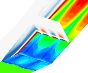
Following the exponential growth, the flow saturates into a new steady state. No supercritical Hopf bifurcation that leads to unsteadiness is found until the end of the simulation. Shown in figure 8(a–c), three wall-normal slices are extracted at x/L = 2.65, 20 and 40 in the saturated stage (tu ∞/L = 29 734). The in-plane streamlines indicate a pair of counterrotating streamwise vortices along the ramp. The contour of the skin friction coefficient in figure 8(d) shows corrugated separation and reattachment lines in a zigzag pattern. Note that the contour is extended to two periods in the spanwise direction. As shown in figure 8(e), the presence of the streamwise vortices elevates the spanwise-averaged Cf in comparison with the base-flow result, leading to better agreement with the experiments and the LES on the ramp.

Figure 8. (a‒c) Contours of the spanwise velocity on three wall-normal planes through x/L = 2.65, 20 and 40 at tu ∞/L = 29 734 superimposed with in-plane streamlines. (d) Contour of the skin friction coefficient at tu ∞/L = 29 734 superimposed with the separation and reattachment lines in black. (e) Distribution of the spanwise-averaged Cf with the spanwise maximum and minimum values marked by the dotted lines. The horizontal dashed lines in (a‒c) mark the isolines of ū/u ∞ = 0.99 obtained from the base-flow solution. Here Reδ = 132 840 and α = 25°.
In the 3-D simulation, the eddy viscosity is allowed to evolve. One may argue that the increasing eddy viscosity may have an unphysical stabilizing effect on the ending of the linear growth and any secondary instabilities after saturation. In this study, we fully rely on the predictive capability of the S–A model for 3-D large-scale flow structures. This is consistent with previous unsteady RANS studies on shock buffet (Crouch et al. Reference Crouch, Garbaruk, Magidov and Travin2009; He & Timme Reference He and Timme2021), where the eddy viscosity was unfrozen throughout the simulations. The effect of different RANS models on the flow bifurcation will be examined in a future study.
4.3. Response to upstream disturbances
We further examine the response of globally stable flows to external disturbances using resolvent analysis. Unless otherwise specified, the forcing is always localized approximately 10δ upstream of the corner to represent upstream disturbances, which extends from the wall to the far field. In fact, the optimal response is found to be insensitive to the forcing location (see Appendix C). Figure 9(a) shows the optimal-gain curves at ωrL/u ∞ = 10−4, 10−3, 10−2 and 10−1 as a function of spanwise wavenumber for the lowRe case at α = 23°. A low-pass feature similar to laminar interactions (Bugeat et al. Reference Bugeat, Robinet, Chassaing and Sagaut2022) is observed. Further lowering the frequency no longer changes the optimal-gain curve. At low frequencies, there are two local maxima in optimal gain at βL = 0 and 0.7. At high frequencies, the maximum optimal gain is found at βL = 1.2. The optimal gain and its frequency-premultiplied value are plotted in figure 9(b–d) as a function of angular frequency at βL = 0, 0.7 and 1.2. Only ωrL/u ∞ ≤ 0.2 is considered, which is at least one order of magnitude lower than the characteristic frequency in the incoming boundary layer and consistent with the assumption of separation of scales. However, this assumption holds less rigorously for the spanwise wavenumber. At the three wavenumbers, the weighted gain has a local maximum at ωrL/u ∞ = 6.5 × 10⁻³, 4.0 × 10⁻⁴ and 7.5 × 10⁻³, respectively. At the three angular frequencies, the optimal response shown in the inset of figure 9(b–d) resembles the corresponding global mode predicted by the GSA, which indicates that the amplification is due to modal resonance.

Figure 9. (a) Optimal gains at different angular frequencies and (b‒d) optimal gains and the frequency-premultiplied values at βL = 0, 0.7 and 1.2 and the corresponding optimal responses at Reδ = 63 560 and α = 23°. Local maxima are indicated by the vertical dashed lines and open circles.
Quantitatively, the 2-D optimal response at ωrL/u ∞ = 6.5 × 10⁻³ is compared with the 2-D shock mode (ωrL/u ∞ = 0 and βL = 0) obtained from the GSA in figure 10(a) by plotting the distributions of the Chu energy density integrated in the wall-normal direction. The Chu energy densities are normalized by their respective maximum values. The global mode is supported by the separation bubble and is thus absent in the incoming boundary layer. The optimal response has a local peak at the forcing location, decreases monotonically along the flat plate and experiences an abrupt increase near the separation point. Inside the separation region, the Chu energy density of the optimal response agrees well with that of the global shock mode. The slight difference downstream of reattachment is likely due to the non-zero frequency of the optimal response and potential non-normalities. A similar comparison is made between the optimal response at ωrL/u ∞ = 4.0 × 10⁻⁴ and βL = 0.7 and the bubble mode at the same spanwise wavenumber in figure 10(b). The almost overlapping Chu energy density distributions downstream of separation confirm that the local maxima of the optimal gain are essentially caused by modal resonance, while both convective-type non-normality (e.g. the Görtler instability) and component-type non-normality (e.g. transient growth of streamwise vortices) are insignificant (Chomaz Reference Chomaz2005).

Figure 10. Distributions of the normalized Chu energy density integrated in the wall-normal direction for (a) the optimal response at ωrL/u ∞ = 6.5 × 10⁻³ and βL = 0 and the shock mode at βL = 0 and (b) the optimal response at ωrL/u ∞ = 4.0 × 10⁻⁴ and βL = 0.7 and the bubble mode at βL = 0.7 at Reδ = 63 560 and α = 23°. The vertical dashed lines mark the separation and reattachment points.
The optimal-forcing profiles corresponding to the optimal responses at ωrL/u ∞ = 6.5 × 10⁻³, 4.0 × 10⁻⁴ and 7.5 × 10⁻³ are plotted in figure 11. The 2-D optimal forcing works as a streamwise momentum pump in the incoming boundary layer, resulting in a periodic variation of the velocity profile. The 3-D forcings are characterized by streamwise vortices with the forcing energy contributed mostly by the spanwise momentum component. The spanwise component has its largest amplitude close to the wall and changes its sign near y/δ = 0.3. Interestingly, part of the forcing is present outside the boundary layer for both the 2-D and 3-D cases.

Figure 11. Optimal forcings at (a) ωrL/u ∞ = 6.5 × 10⁻³ and βL = 0, (b) ωrL/u ∞ = 4.0 × 10⁻⁴ and βL = 0.7 and (c) ωrL/u ∞ = 7.5 × 10⁻³ and βL = 1.2 at Reδ = 63 560 and α = 23°.
Of particular interest is the 2-D optimal response as an excitation of the shock mode by external disturbances. Recall that the base flow is always stable to 2-D perturbations, which allows resolvent analysis at different Reynolds numbers and ramp angles. The resulting weighted gain is presented in figure 12. For the lowRe case, the angular frequency associated with the low-frequency peak decreases as α is increased. At α = 25°, increasing the Reynolds number further decreases the frequency. When non-dimensionalized using the length of the separation region, the frequencies with different interaction strengths collapse onto a universal value of f Lsep/u ∞ = 0.015, which is consistent with the findings of Dussauge et al. (Reference Dussauge, Dupont and Debiève2006).

Figure 12. Premultiplied optimal gain at βL = 0 as a function of (a) ωrL/u ∞ and (b) f Lsep/u ∞ at different ramp angles. Local maxima are indicated by the vertical dashed lines. Solid lines, Reδ = 63 560; dash-dotted lines, Reδ = 132 840.
To reveal its nonlinear behaviour, a 2-D unsteady RANS simulation is performed, which is initialized using the 2-D base flow for the highRe case at α = 25°. The base flow is perturbed by the optimal forcing at f Lsep/u ∞ = 0.015. The forcing amplitude is set to  $0.01{\rho _\infty }u_\infty ^2/L$. The time step is also 20 ns. The wall pressure is monitored at the base-flow separation point (x/L = −16.75), as shown in figure 13(a). The signal exhibits the well-known intermittent feature with the pressure oscillating between the free-stream pressure and the pressure behind the separation shock. The separation shock undergoes a back-and-forth motion (see the supplementary movie available at https://doi.org/10.1017/jfm.2023.687) with an intermittent region of approximately 0.6δ. The locations of the separation and reattachment points are shown in one cycle in figure 13(b). The bubble undergoes a breathing motion with the separation and reattachment points moving in opposite directions.

Figure 13. Time histories of (a) wall pressure at the base-flow separation point and (b) locations of the separation and reattachment points for the highRe case at α = 25°. The dashed lines in (b) indicate the base-flow solution.
A more informative simulation is performed with the 2-D base flow perturbed by white noise at the same forcing location as the resolvent analysis for the highRe case at α = 25°. The random forcing is added to the right-hand side of the momentum equations with an amplitude of  $0.1{\rho _\infty }u_\infty ^2/L$ and updated every 2500 steps to avoid violating the assumption of separation of scales. Consequently, the highest introduced frequency is 20 kHz (ωrL/u ∞ = 0.2). The simulation is run for 50 ms (tu ∞/L = 30 973) with a time step of 20 ns. Figure 14(a) shows the wall pressure history at the base-flow separation point, which also has an intermittent behaviour. Spectral analysis is performed for the pressure signal between tu ∞/L = 6195 and 30 973 with Welch's method (Welch Reference Welch1967) to calculate the power spectral density (PSD) shown in figure 14(b). The signal is divided into three segments with 50% overlap. A Hann window is used for weighting the data. The frequency-premultiplied PSD peaks at f Lsep/u ∞ = 0.015. This also suggests that the forcing profile is insignificant for modal resonance, which amplifies the low-frequency component of any upstream disturbances and results in a back-and-forth shock motion.

Figure 14. (a) Time history of wall pressure at the base-flow separation point and (b) the corresponding PSD for the highRe case at α = 25°.
Additional RANS simulations are performed for the 3-D optimal responses at βL = 0.7 and 1.2 and other values of βL for the lowRe case at α = 23°. The forcing amplitude is set to  $0.01{\rho _\infty }u_\infty ^2/L$. Figure 15 presents the contours of Cf at four instants with nearly equal intervals in one cycle at ωrL/u ∞ = 7.5 × 10⁻³ and βL = 1.2. Note that the contours are extended to two periods in the spanwise direction. As expected, the saturated flow resembles that in § 4.2 featuring corrugated separation and reattachment lines and counterrotating streamwise vortices along the ramp. However, these vortices are not fixed in the spanwise direction but undergo a spanwise meandering motion (see the supplementary movie), which is reminiscent of the numerical results of Priebe et al. (Reference Priebe, Tu, Rowley and Martin2016) and Pasquariello et al. (Reference Pasquariello, Hickel and Adams2017). The contour of spanwise velocity on an x–y plane through z/L = 4.5 at tu ∞/L = 1229 further confirms the excitation of the bubble mode identified by the GSA (see figure 16).

Figure 15. Contours of the skin friction coefficient at tu ∞/L = (a) 1229, (b) 1413, (c) 1659 and (d) 1844 superimposed with the separation and reattachment lines in black for the lowRe case at α = 23°.

Figure 16. (a) Spanwise velocity contour on an x–y plane through z/L = 4.5 at tu ∞/L = 1229 and (b) real part of w′ of the bubble mode at βL = 1.2 obtained from the GSA for the lowRe case at α = 23°. The dashed lines in (b) indicate the isoline of ū/u ∞ = 0.99 and the dividing streamline.
5. Conclusions
The low-frequency, large-scale motions in STBLIs over a compression corner are examined using GSA and resolvent analysis based on the assumption of separation of scales.
The GSA reveals that the 2-D base flow becomes unstable to 3-D perturbations as the ramp angle is beyond a critical value. Only a stationary unstable mode is identified, whose spanwise wavelength scales with the bubble size. At large spanwise wavenumbers, this mode is mostly confined to the separation bubble and the reattached boundary layer. At small spanwise wavenumbers, this mode manifests itself as a coupling between the separation shock and the separated shear layer. The GSA predictions are confirmed by a 3-D numerical simulation, where no supercritical Hopf bifurcation that leads to unsteadiness is found. The saturated flow exhibits a spanwise alternating expansion/contraction of the separation bubble and counterrotating streamwise vortices downstream of the corrugated reattachment line. For globally stable flows, the resolvent analysis identifies 2-D and 3-D local maxima in optimal gain due to modal resonance between external disturbances and the leading global mode, while the Görtler instability makes no evident contribution. A numerical simulation reveals that the 2-D optimal response is in the form of a large-scale, back-and-forth shock motion accompanied by a breathing bubble. The 3-D optimal responses all exhibit counterrotating streamwise vortices that meander in the spanwise direction with a range of frequencies and spanwise wavenumbers.
This study suggests that the low-frequency shock motion in STBLIs is caused by the excitation of an intrinsic mode by extrinsic disturbances in line with the mathematical models of Plotkin (Reference Plotkin1975) and Touber & Sandham (Reference Touber and Sandham2011), while the streamwise vortices are due to either global instability or modal resonance.
Supplementary movies
Supplementary movies are available at https://doi.org/10.1017/jfm.2023.687.
Funding
This work is supported by the Hong Kong Research Grants Council (no. 15206519 and no. 25203721) and the National Natural Science Foundation of China (no. 12102377).
Declaration of interests
The author reports no conflict of interest.
Appendix A. Verification of the RANS simulations and stability analysis
Figure 17 compares the distributions of Cf and the eigenvalue spectra at βL = 0.36 obtained with two meshes including 500 × 200 (coarse) and 700 × 300 (fine) at Reδ = 132 840 and α = 25°. The coarse mesh is sufficient for both base-flow computation and stability analysis. Figure 18 shows the time history of the Euclidean norm of the density residual in the base-flow simulation at Reδ = 132 840 and α = 25°. The density residual is normalized by its value in the first iteration. In figure 19, the effect of the size of the computational domain is examined. As long as the far-field and outflow boundaries are far enough away from the separation bubble, the stability analysis results are unchanged.

Figure 17. (a) Distributions of the skin friction coefficient and (b) eigenvalue spectra at βL = 0.36 obtained with the coarse and fine meshes at Reδ = 132 840 and α = 25°.

Figure 18. Time history of the Euclidean norm of the density residual at Reδ = 132 840 and α = 25°.

Figure 19. (a) Schematic of two computational domains of different sizes and (b) eigenvalue spectra at βL = 0.36 obtained with different domains at Reδ = 132 840 and α = 25°. The dashed lines in (a) indicate the isoline of ū/u ∞ = 0.99 and the dividing streamline. The horizontal and vertical dashed lines in (b) indicate zero growth rate and zero angular frequency, respectively.
For the 3-D RANS simulation of the highRe case at α = 25° without external disturbances, two additional simulations are considered: the number of grid cells in the spanwise direction is doubled, and the time step is halved. To save computational cost, the second simulation starts from a baseline flow field in the linear stage, and both simulations are run for 30 ms (tu ∞/L = 18 584). The time histories of σw at x/L = 2.65 are compared in figure 20. The flow evolution remains unchanged.

Figure 20. Time histories of σw at x/L = 2.65 obtained with different levels of grid refinement and time steps at Reδ = 132 840 and α = 25°.
Appendix B. Effect of RANS modelling
A new base flow is computed using Wilcox's k–ω model (Wilcox Reference Wilcox2008) with a stress-limiter coefficient of 0.9 at Reδ = 132 840 and α = 25°. The resulting distribution of Cf is compared with that predicted by the S–A model in figure 21. Good agreement is obtained, except that the k–ω model predicts an elevated skin friction on the ramp. The frozen eddy-viscosity approach (cf. Carini et al. Reference Carini, Airiau, Debien, Léon and Pralits2017) is adopted in the GSA. In other words, the GSA solver for laminar flow (Hao et al. Reference Hao, Cao, Wen and Olivier2021) is used with the effective viscosity equal to the sum of the molecular and eddy viscosities. As a comparison, GSA is also performed on the base flow predicted by the S–A model using the frozen eddy-viscosity approach. For both cases, only a stationary unstable mode is captured. The growth rate curves as a function of βL are compared in figure 22. When the eddy viscosity is frozen, the modal coalescence phenomenon is absent, and the 2-D mode becomes globally unstable. This suggests that the 2-D unstable mode is likely an artefact of the frozen eddy-viscosity approach. Nonetheless, the obtained shapes of the leading mode at βL = 0 and 0.36 in figure 23 clearly exhibit the same features as those in figure 3, which indicates that the dynamics revealed in this study is insensitive to RANS modelling.

Figure 21. (a) Skin friction coefficient and (b) wall pressure distributions predicted by the S–A and k–ω models at Reδ = 132 840 and α = 25°. The horizontal dashed line indicates zero skin friction.

Figure 22. Growth rates of the most unstable mode as a function of βL predicted by different RANS models at Reδ = 132 840 and α = 25°. The horizontal dashed line indicates zero growth rate.

Figure 23. (a,b,d,e) Real parts of u′ and w′ of the leading mode at βL = 0.36 and (c, f) real part of u′ of the leading mode at βL = 0 predicted by different RANS models with the frozen eddy-viscosity approach at Reδ = 132 840 and α = 25°. The dashed lines indicate the isoline of ū/u ∞ = 0.99 and the dividing streamline.
Appendix C. Effect of the forcing location
Figure 24 compares the optimal-gain curves at ωrL/u ∞ = 10−4 obtained with different forcing locations. In the baseline case, the forcing is localized 10δ upstream of the corner. As a comparison, the forcing is implemented in the entire domain. Note that the optimal gains are normalized using their respective maximum values. The good agreement indicates that the current resolvent analysis results are independent of the forcing location. The STBLIs under consideration preferably amplify upstream disturbances, while downstream disturbances are much less effective in causing large energy amplification.

Figure 24. Normalized optimal gains at ωrL/u ∞ = 10−4 as a function of βL with different forcing locations at Reδ = 63 560 and α = 23°.


 Open access